1. Hand-eye Calibration Tool

1.1. What is Hand-eye Calibration?

Many robot vendors provide TCP (Tool Center Point) calibration and UF (User Frame) calibration functionality in the teaching pendant, making it possible to interact with objects using an EOAT (End Of Arm Tool). However, when robots work with vision sensors (snapshot/profile sensors), the calibration requires solving homogeneous transform equations because the origin of the sensor coordinate frame is not tangible.

This toolbox provides a handy way to perform TCP/UF calibrations in the following scenarios:

TCP Calibration: A snapshot/profile sensor is mounted on an active robot. The transformation from the robot flange to the sensor origin is calculated.
UF Calibration: A snapshot/profile sensor is mounted on the wall, ceiling, or other fixtures. The transformation from the robot base to the sensor origin is calculated.

1.2. Method Overview

A: Input Robot pose expressed in the robot base coordinate frame
B: Input Calibration artifact position expressed in the sensor coordinate frame.
X: Output Sensor coordinate expressed in the robot tool frame  (TCP Calibration).
Y: Output Sensor coordinate expressed in the robot base coordinate frame  (UF Calibration).

In basic form, the calculation requires 9 different combinations of A and B to get either X or Y: 9 x (A + B) = X or Y

TCP Calibration:

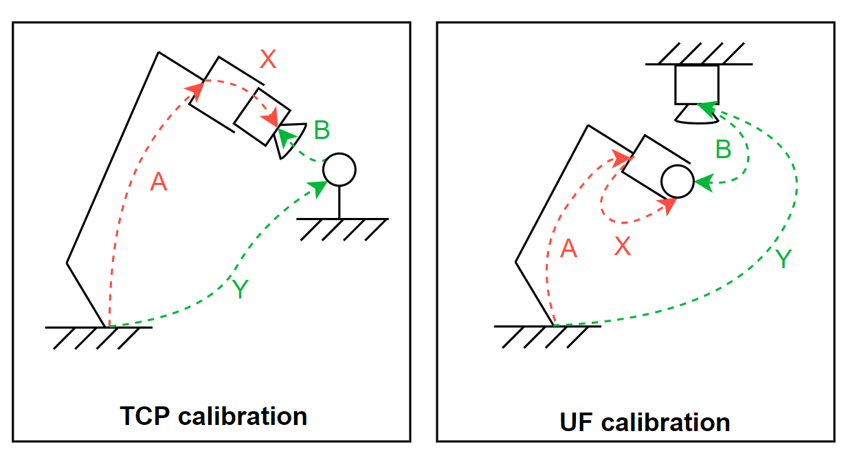
TCP calibration calculates the transformation from the robot flange to the sensor origin, denoted as X. The sensor is mounted on the robot flange and a calibration artifact is placed on a flat surface. The algorithm requires the sensor to view the artifact using at least 6 different poses (or 9 poses if possible). The user needs to record both the robot pose A in the robot base coordinate frame and the position of the artifact B in the sensor coordinate frame.

UF Calibration:

UF calibration calculates the transformation from the robot base to the sensor origin, denoted as Y. The sensor is mounted on the wall/ceiling/other fixtures, and the calibration artifact is mounted on a robotic flange. The algorithm requires the sensor to view the calibration artifact using at least 6 different poses (or 9 poses if possible). The user needs to record both the robot pose A in the robot base coordinate frame and the position of the artifact B in the sensor coordinate frame.

1.3. Calibration Procedure

1.3.1. Calibration Steps

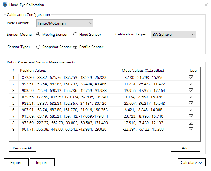
Select the format of robot poses being used from Pose Format.
Select moving sensor from Sensor mount for TCP Calibration, which sensor moves with the robot. Select fixed sensor from Sensor mount for UF Calibration, which sensor is fixed at a location.
Select Snapshot Sensor or Profile Sensor from Sensor Type. A snapshot sensor can capture a point cloud (XYZ) in its FOV, while a profile sensor captures a profile (XZ) in its FOV.
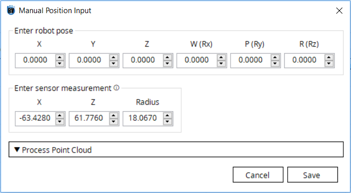
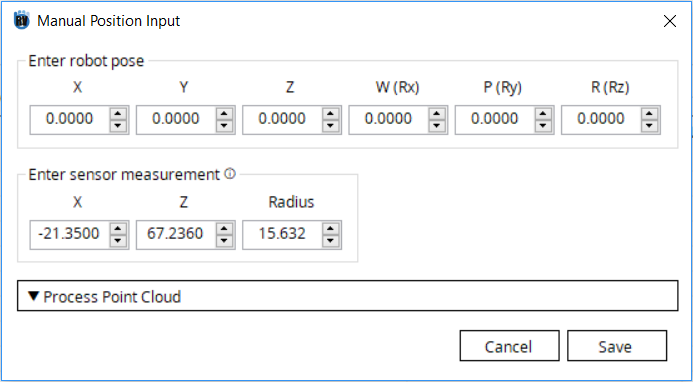
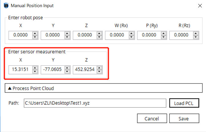
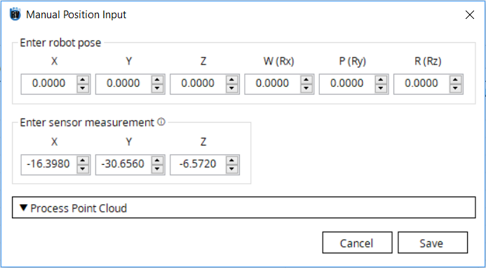
Move the robot to a pose. Gather the pose information from the robot and the position of the calibration target in the sensor’s frame. Click Add on the bottom-right corner. Input the robot poses and the sensor measurement under correspondingly.

When the labels in Enter sensor measurement are X, Y and Z, the center position of the target in the sensor’s frame is required.

When the labels in Enter sensor measurement are X, Z and Radius, enter the 2D center position of the profile circle in X and Z, and enter the radius of the profile circle in radius.

Note

All X,Y,Z and Radius unit is mm. Refer to Sensor Measurement Collection for additional info.

5. Repeat step 4 for 9 times (minimum 6 times if there is robot motion constraint). When selecting the robot poses, try to avoid poses with close proximity or poses with close camera orientations. The animation below shows a good example of 9 poses.

Note

In the animation above, the user needs to change the value of R (the 6th axis) in each pose.

That is because the poses in the gif animation can only guarantee the variance in XYZWP (the 1st-5th axes).

Attention

Make sure when recording the robot positions that the coordinates are with respect to the robot base and robot flange (a User Frame of 0 and Tool Frame of 0).

Click Calculate>> and view the final result.

When the calibration configuration has been setup and all calibration data has been input, click on the Calculate>> button to see the calibration result.

The calibration data as well as the calibration result can be exported for further reference by clicking on Export button. The exported file can be either XML file or CSV file. When XML file is selected, all the configuration, calibration data and the calibration result (if a calibration has been performed) will be saved. When CSV file is selected, only the calibration data will be saved.

The Import button can be used to import an exported file which is either an XML file or CSV file.

1.3.2. Sensor Measurement Collection

TCP/UF calibration requires a minimum of 6 robot poses (Recommended to have 9 positions) to solve the homogeneous transform equations. Although the selection of poses is mostly arbitrary, viewing the calibration target from different angles can generate a more unbiased result. It is highly recommended that the sensor orientation at each pose have an angle difference of at least 15 degrees.

1.3.2.1. Profile Sensor Measurement

When a Profile Sensor is selected. Choose the Calibration Target to be used. There are three target options: BW Sphere, Customized Sphere, and Other.

When obtaining positions, the profile laser line should be located on only 1 half of the artifact (sphere).

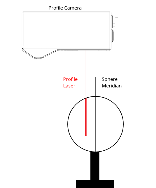
In the above image all measurments should be located on left side of the sphere center line. It does not matter which side is being measured just as long as all measurments are taken from that same side. It is important that no profile measurments are taken at the max radius of the sphere.

Note

The calibration artifacts should have the geometry that when the 3D sensor take images from different orientation, the calculated target center is always the same point.

BW Sphere : A Bluewrist-made high precision sphere with special surface coating for high accuracy calibration.
Customized Sphere: DIY sphere by user
Other: Any calibration target that user needs to provide the center of the target

If Customized Sphere is selected as the Calibration Target. Also input the radius of the sphere in Target Radius.

1.3.2.1.1. Gocator

Currently, Gocator 2xxx series is supported.

Use Gocator web interface, adjust the Scan tab settings so the laser profile on the BW sphere target is in the field of view.

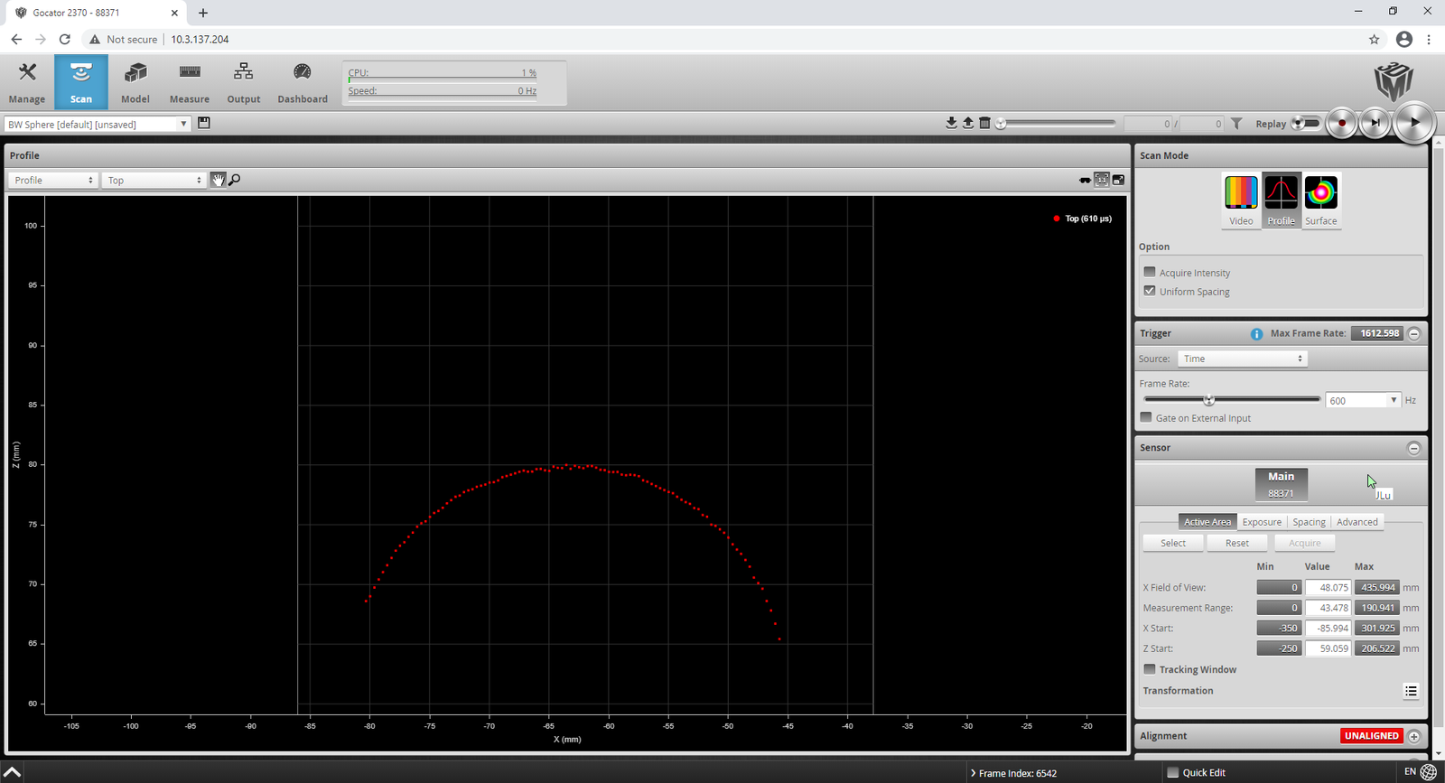
Select Measure tab, use Profile Circle tool and get the X, Z, Radius measurement.

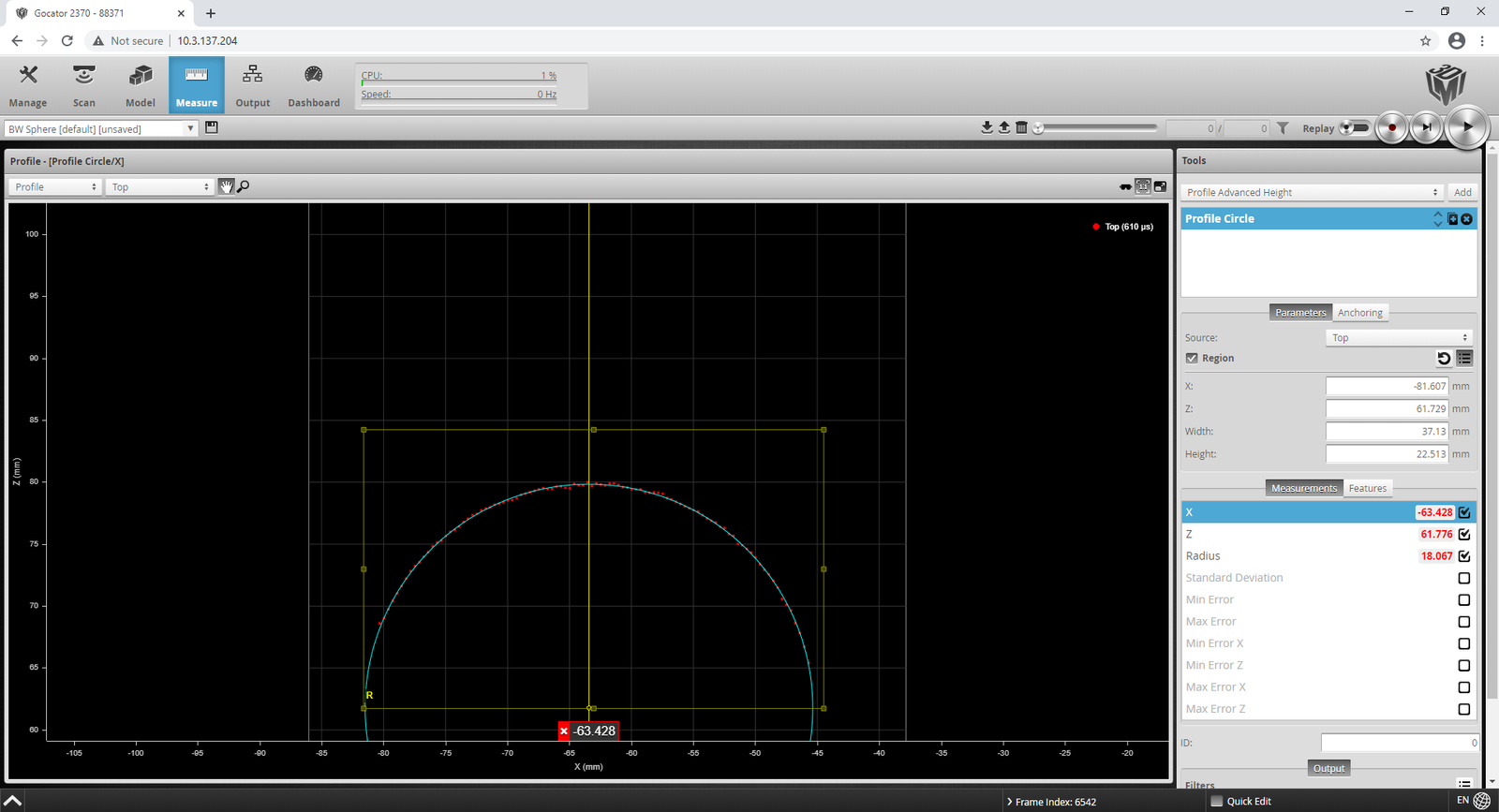
Enter the X, Z, Radius measurement in the corresponding robot pose.

1.3.2.1.2. Keyence

Currently, Keyence LJ-V7000 series is supported.

In LJ-Navigator software interface, adjust settings in the Imaging setting tab so the laser profile on the BW sphere target is in the field of view.

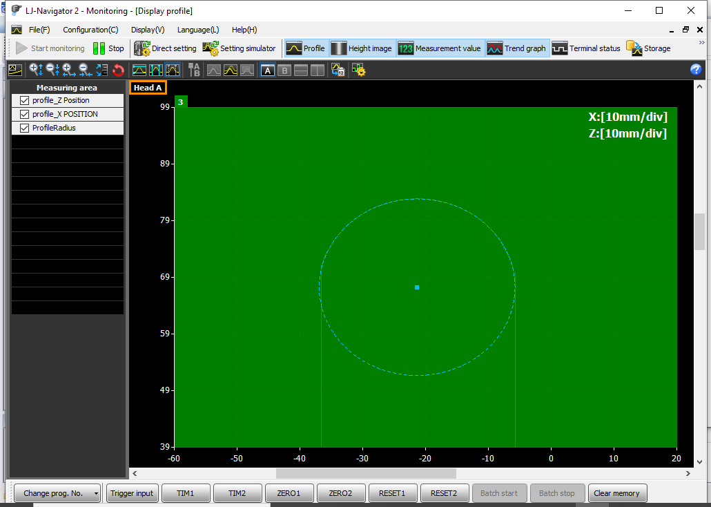
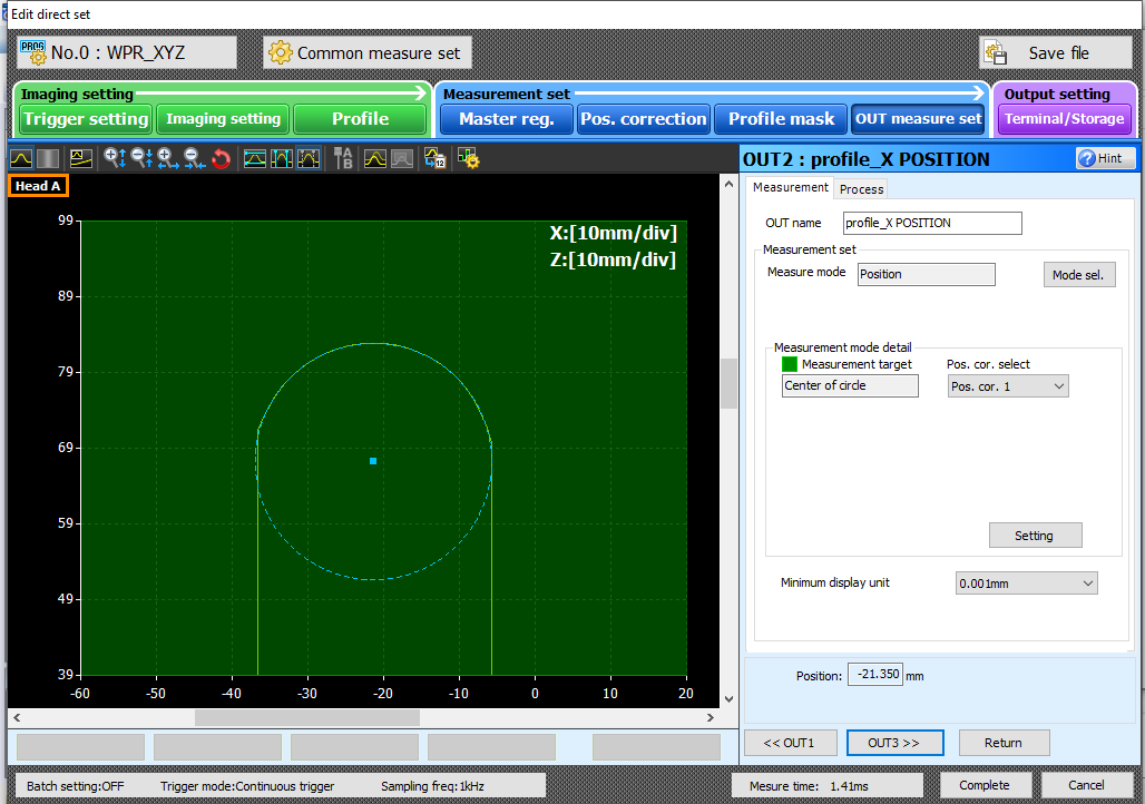
Select OUT Measure set tab, add Position in Measure Mode, this provide the profile_X Position measurement.

Select OUT Measure set tab, add Height in Measure Mode, this provide the profile_Z Height measurement.

Select OUT Measure set tab, use R Measurement in Measure Mode, this provide the Radius measurement.

Enter the Position (X), Height (Z), Radius measurement in the corresponding robot pose.

1.3.2.1.3. Wenglor

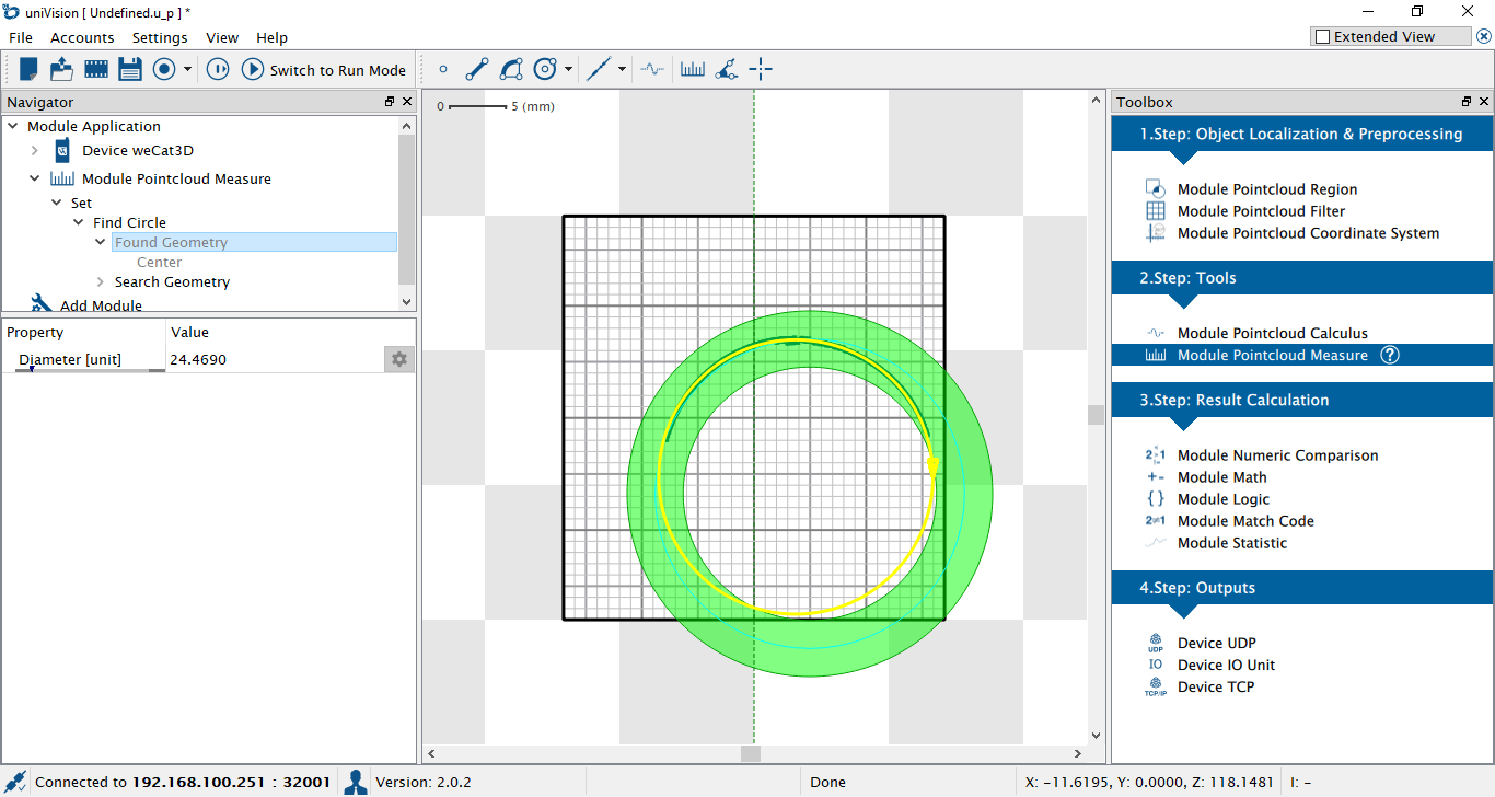
In uniVision software interface, adjust settings so the laser profile on the BW sphere target is in the field of view.

Use Module Pointcloud Measure, add Find Circle, this provide the Diameter measurement.

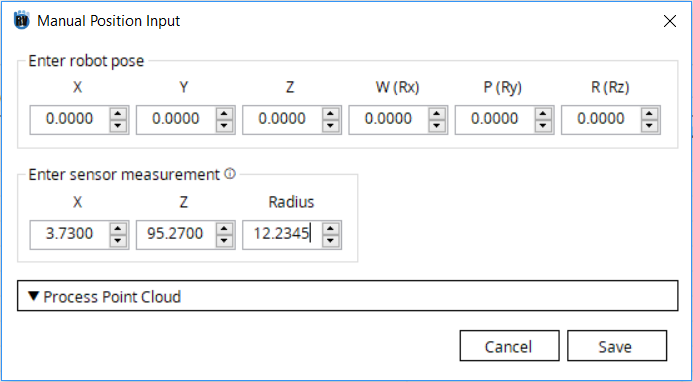
Select Center under Found Geometry, this provide the Origin measurement. The first value is X and the third value is Z measurement.

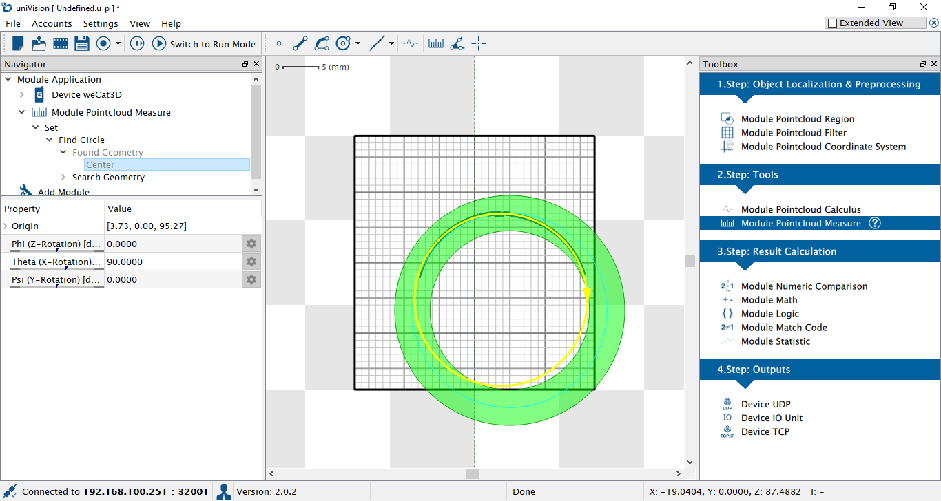
Enter the X, Z, Diameter/2 in the corresponding robot pose.

1.3.2.2. Snapshot Sensor Measurement

When a Snapshot Sensor is selected, the tool box provides a built-in point cloud processing tool for getting sensor measurement directly from the point cloud taken by the sensor. Only BW Sphere and Customized Sphere are supported at moment.

When entering the robot pose and sensor measurement, click Process Point Cloud to expand the window. Click Load PCL to load the point cloud file taken by the sensor. The point cloud file will be loaded into the point cloud viewer. For instructions on how to save point cloud, refer to each sensor section respectively.

Clearing the point cloud: In the PLC Trimming group, click Select Box. Click and drag mouse left click to draw a rectangular box, the selected point cloud will be marked red. Clicking Crop Selected will remove the selected points, and clicking Keep Selected will remove the unselected points while keeping only the selected points.

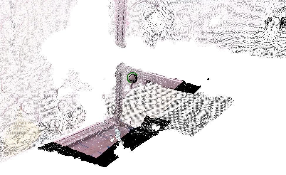
When there are only points of the calibration target in the point cloud, in the Feature Extraction group, click Fit Sphere to extract the sphere target in the point cloud. The result will be shown in the textbox and the fitted sphere will be drawn in the point cloud viewer.

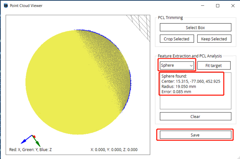
After finding the fitted sphere, click Save and the result will be entered into the sensor measurement automatically.

1.3.2.2.1. Photoneo

The following steps illustrate how to collect point cloud using Photoneo software.

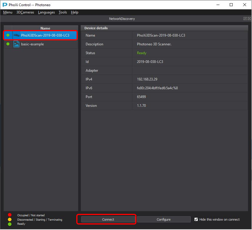
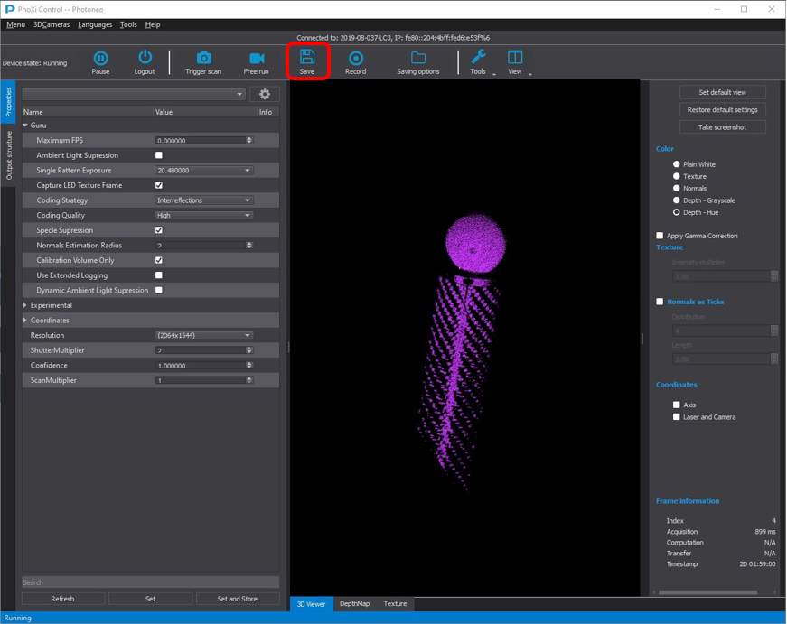
Open PhoxiControl software and wait until the sensor becomes available under Name in NetworkDiscovery page.

Click Trigger Scan to capture the image of the calibration target. Adjust the parameters on the left column to improve the point cloud quality. Usually the default values of the parameters work very good in most setups, but sometimes they still need to be tuned to reduce the reflections and counterbalance the ambient light.

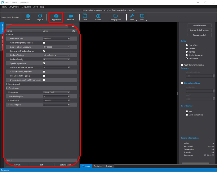
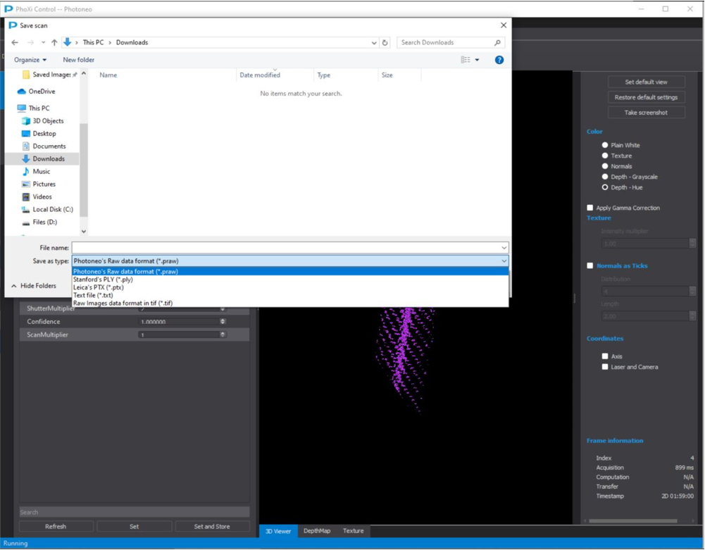
Click Save

Save file into .xyz format

1.3.2.2.2. Visionerf

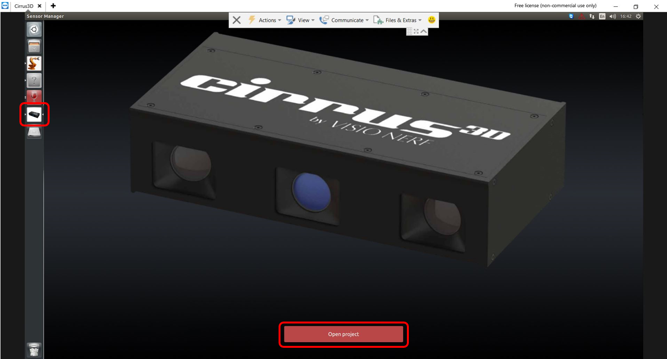
The following steps illustrate how to collect point cloud using Visionerf software.

Connect the sensor through TeamViewer. Select Sensor Manager from the left column and click Open project

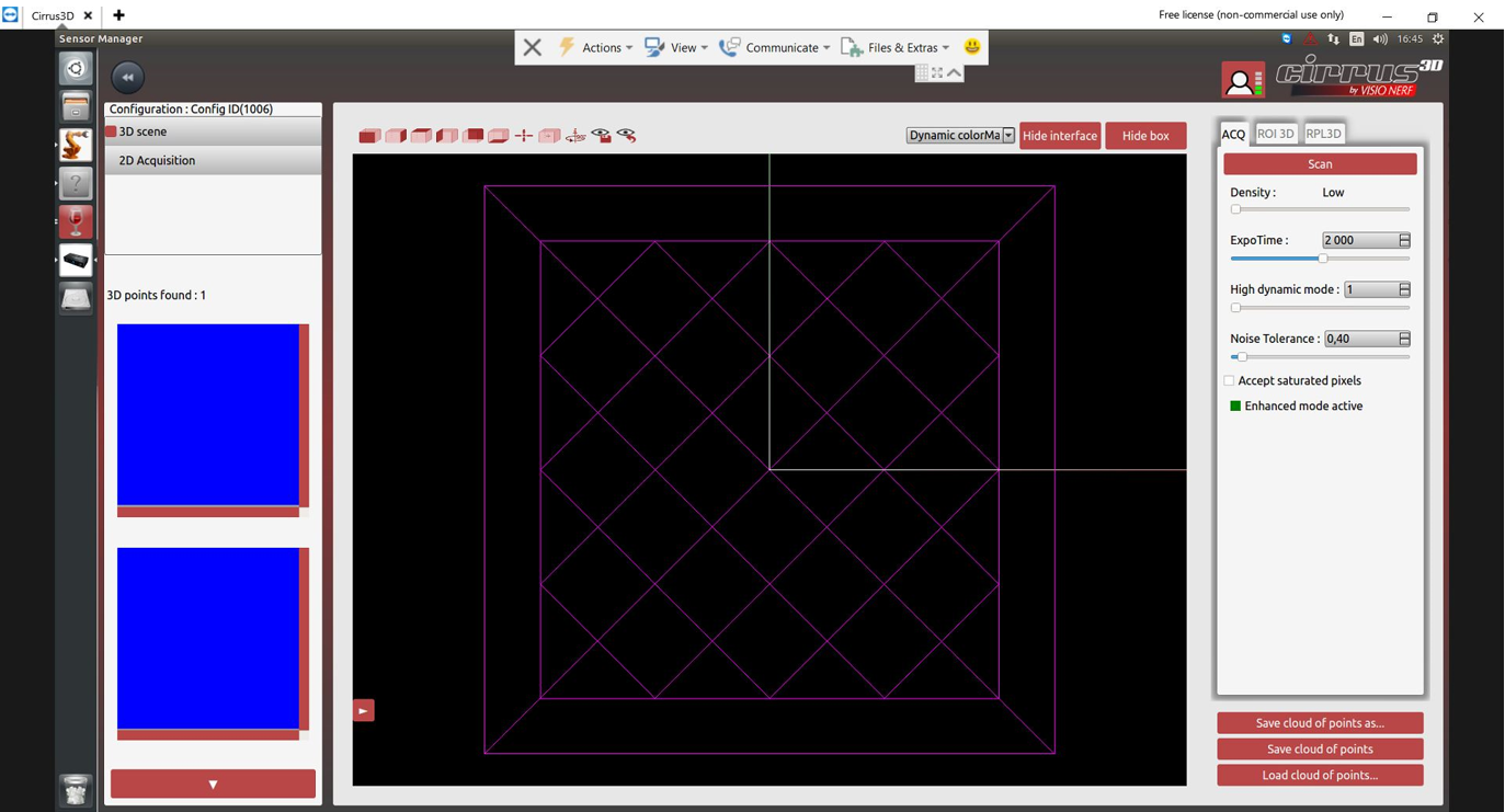
Select a configuration profile under Acquisition on right hand side column, then click Edit

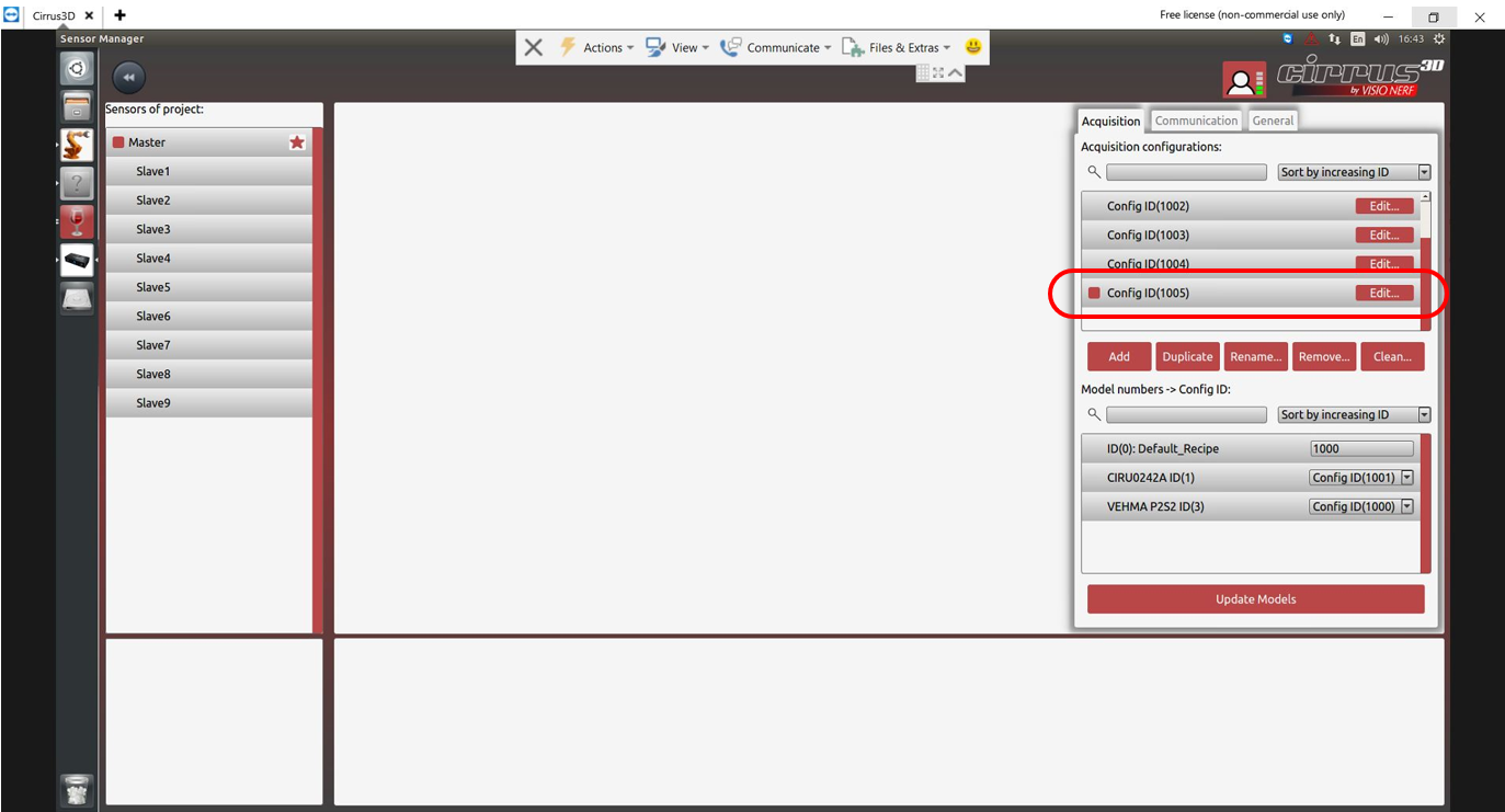
Adjust parameters such as Density, ExpoTime, High dynamic mode and Noise Tolerance to improve the point cloud quality. For example, for Cirrus 300, the following parameters work well with BW Sphere

<Density: High>

<ExpoTime: 5000>

<High dynamic mode: 3>

<Noise Tolerance: 0.6>

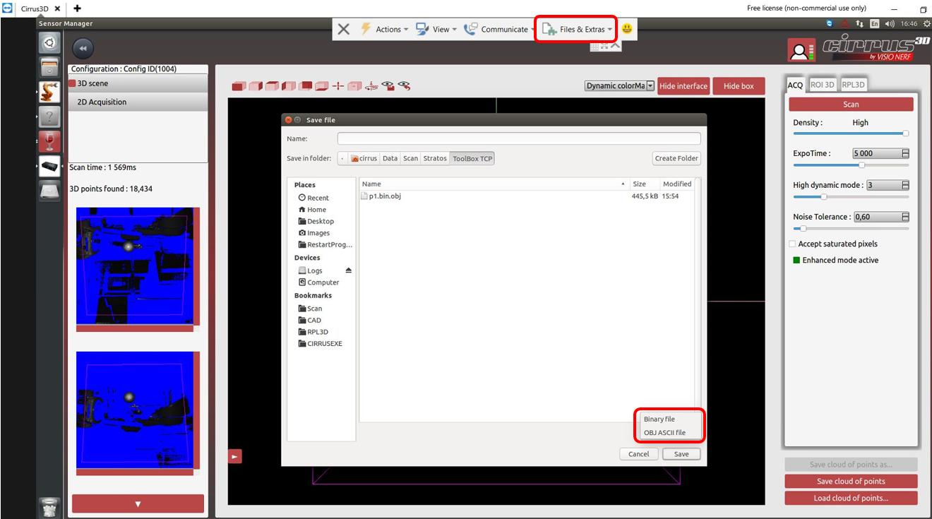
Click Save cloud of points as

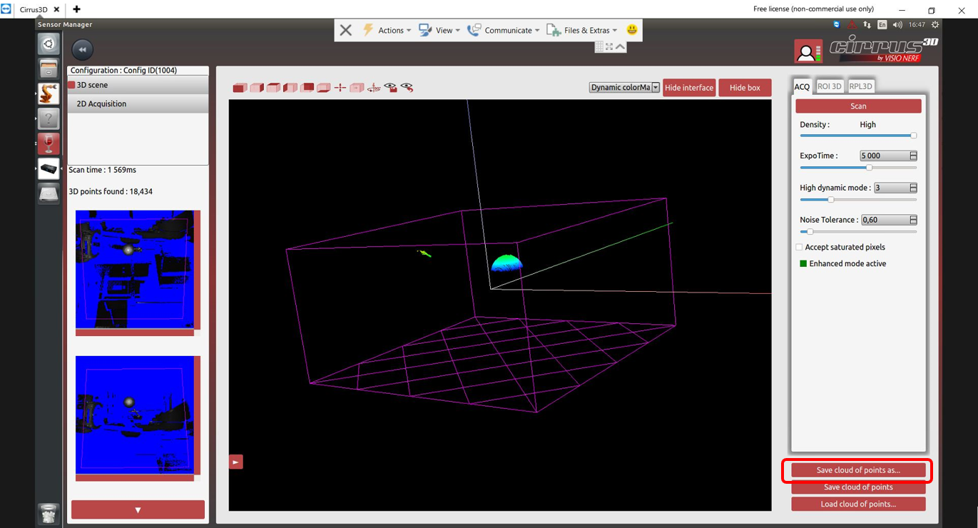
Choose the Binary File format and save the point cloud in the desired directory. Use file transfer wizard (top of the page) of TeamViewer to transfer the point clouds to your PC.

1.3.2.2.3. Wenglor

The following steps illustrate how to collect point cloud using Wenglor software.

Download and install the SDK ShapeDrive_Essential_1.0.0.zip from the official website.
Config the 10-Gigabit/1-Gigabit Network Connection by following the Operating_Instructions_<SensorModel>.pdf available on the official website.
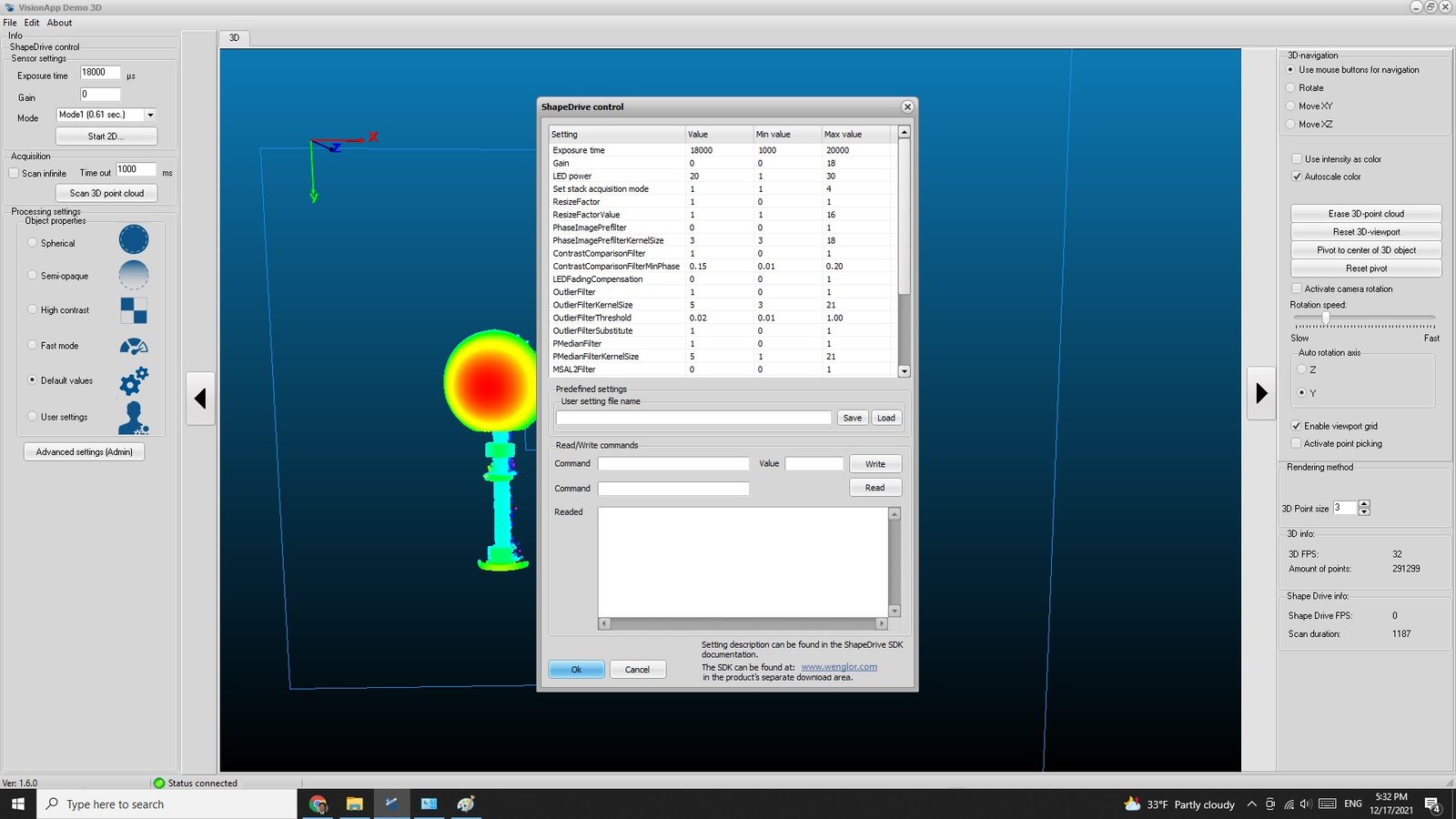
Open Wenglor software VisionApp Demo3D and connect to the sensor. Users may need to load the sensor database (available on their official website) prior to connecting to the sensor.

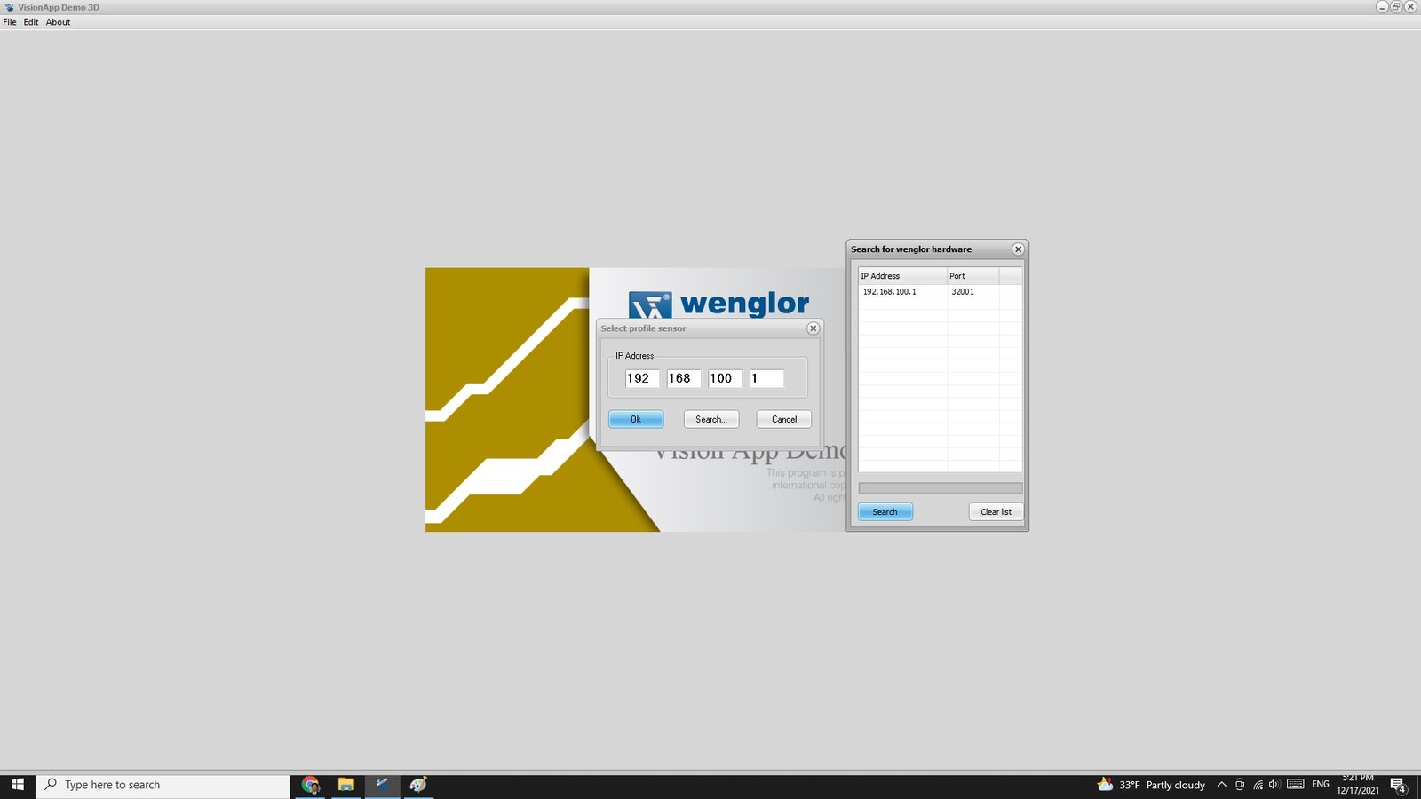
Users can switch between the 2D and the 3D viewes using the acquisition buttons on the left.

Adjust the exposure time and other parameters.

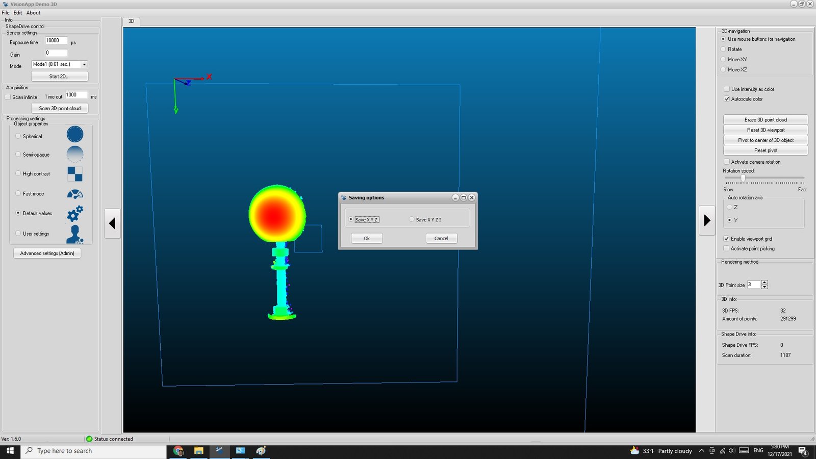
Save the PCL as .xyz format.

1.3.2.2.4. Zivid

The following steps illustrate how to collect point cloud using Zivid software.

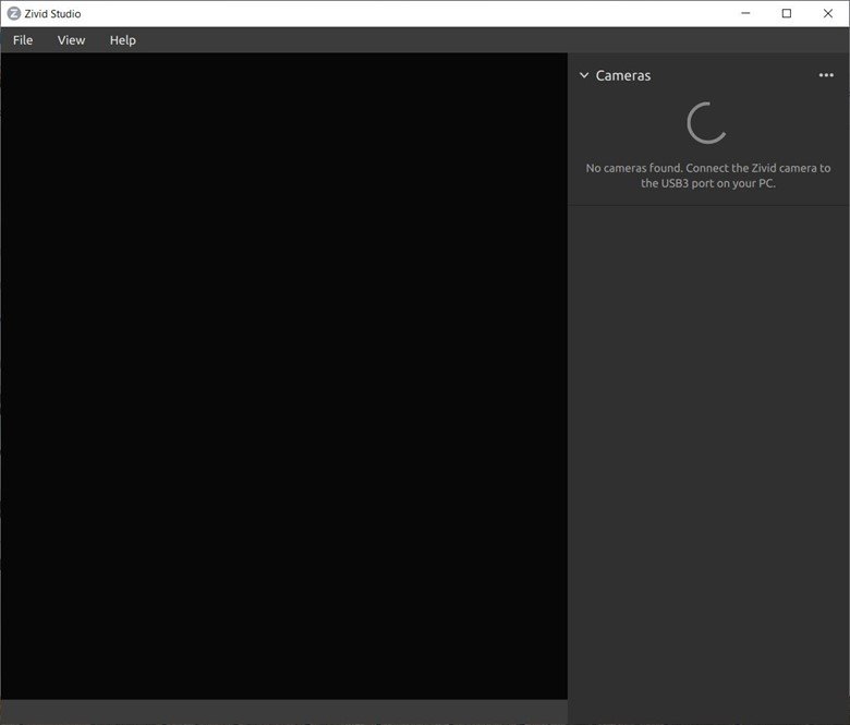
Open Zivid Studio software and the application will automatically search and connect to the sensor.

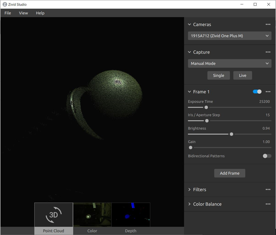
Choose Manual Mode under Capture. Add first frame and adjust Brightness so most of the calibration artifact surface is visible.

Add second frame, adjust Brightness so the complete point cloud of the calibration artifact surface is shown. It is suggested to set one frame’s brightness to high and the other frame’s brightness to low.

Goto File and click Export

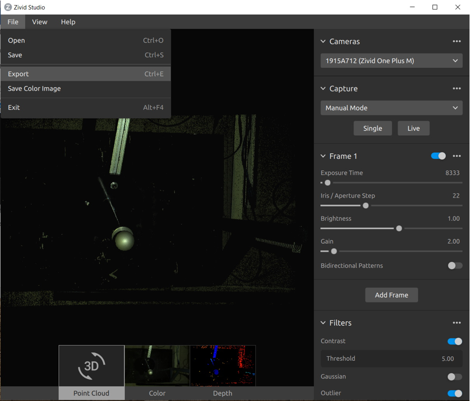
Save file into .xyz format

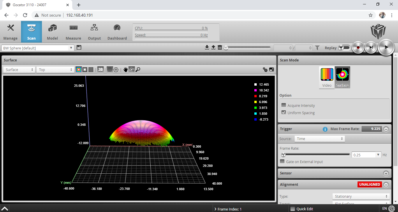
1.3.2.2.5. Gocator

For Gocator, the user can either choose to use Process Point Cloud tool, or use Gocator Measurement function to calculate sphere center.

Use Gocator web interface, adjust the Scan tab settings so the BW sphere target is in the field of view.

Select Measure tab, use Surface Bounding Box tool and get the Center X, Y, Z measurement

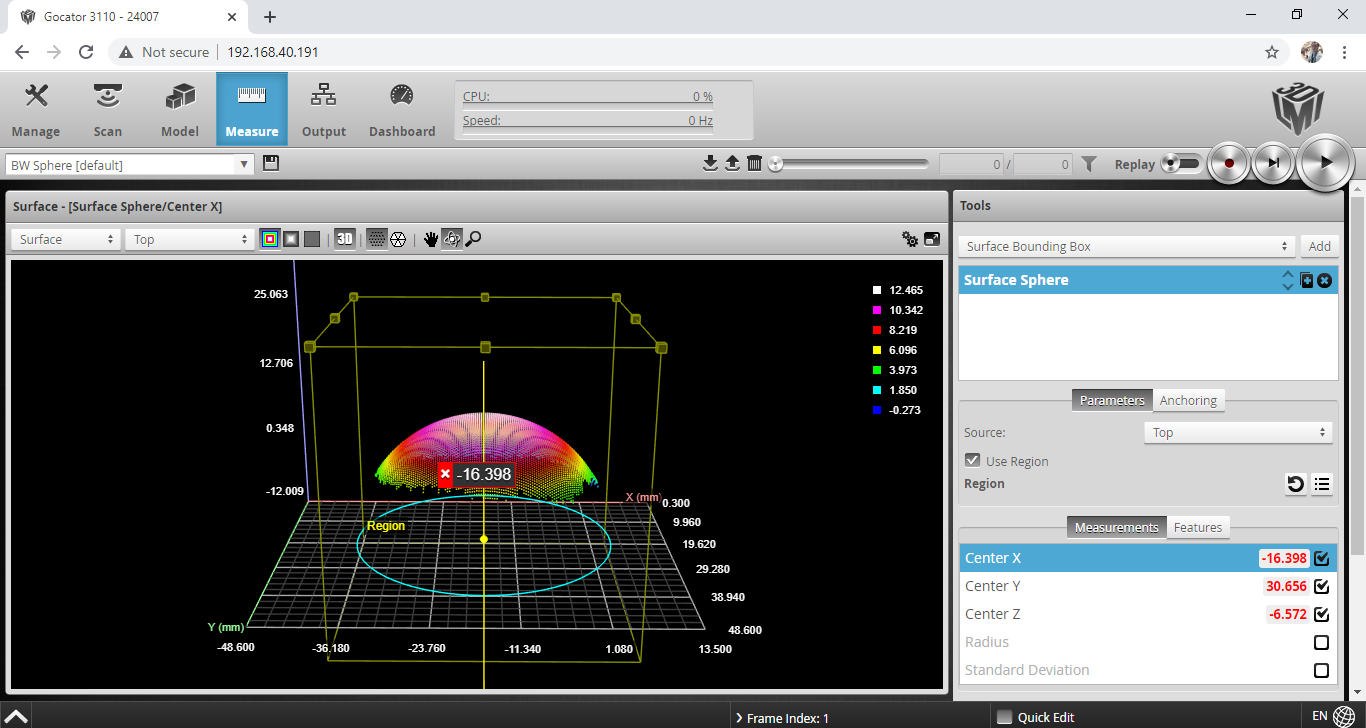
Enter the Center X, Y, Z measurement in the corresponding robot pose.

Warning

The LMI Gocator 3xxx sensors use left-hand coordinates in the web interface, but our toolbox ONLY supports sensors that use right-hand coordinates.

Therefore, the user must invert the sign of y whenever you use the values from the LMI web interface to read the values from a Gocator 3xxx series sensor.

1.3.3. Analyzing Calibration Results

1.3.3.1. Calibration Result

The final calibration result is given in the format same as the input robot pose format. Unblink3D supports following formats from robot vendors:

ABB Quaternion X,Y,Z,q1,q2,q3,q4
ABB Euler angle (deg) X,Y,Z,Ez,Ey,Ex
FANUC Euler angle (deg) X,Y,Z,W,P,R
KUKA Euler angle (deg) X,Y,Z,A,B,C
Motoman Euler angle (deg) X,Y,Z,Rx,Ry,Rz
NACHI Euler angle (deg) X,Y,Z,r,p,y
Universal Robots axis angle RPY (deg)
Universal Robots axis angle RPY (rad)
Universal Robots rotational vector (deg)
Universal Robots rotational vector (rad)

1.3.3.2. Calibration Error

The calibration error indicates the overall error (in mm) of the hand-eye calibration.

The error induced by each pose is also given in the table. The error with red background indicates a large error, and error with white background indicates a small error. One can deselect a pose depending on the error at each pose by unchecking the checkbox in the Use column in the calibration data and recalculate the new calibration result.

In addition to the final result, the window also shows the final calibration error (mm) and the calibration error at each pose (mm). The calibration error at each pose can be used to find out the outlining data. The user is encouraged to review those outlining data points or eliminate them if necessary.

Attention

Acceptable Calibration Error

When the user performs a TCP/UF calibration with an industrial-grade 3D vision sensor, it is ideal to have an error of less than 1.0 mm, but one with 2.0 mm is still acceptable. It is strongly recommended to review the dataset when the error is higher than the threshold.

When the user perform a TCP/UF calibration with a Time of Flight (TOF) camera, or Depth-sensing camera, it might yield a calibration error of around 5.0 mm.

1.4. Examples

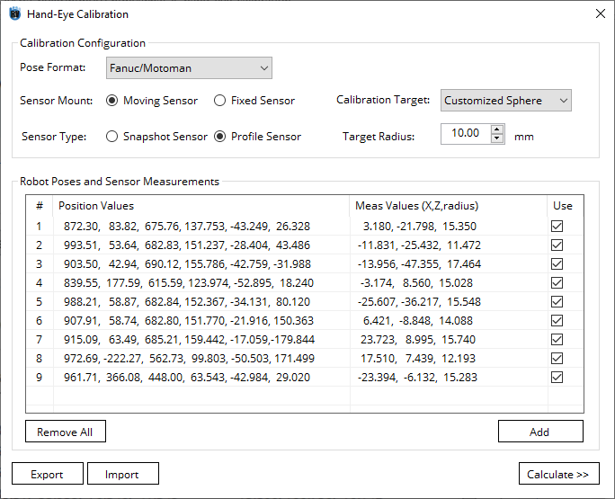
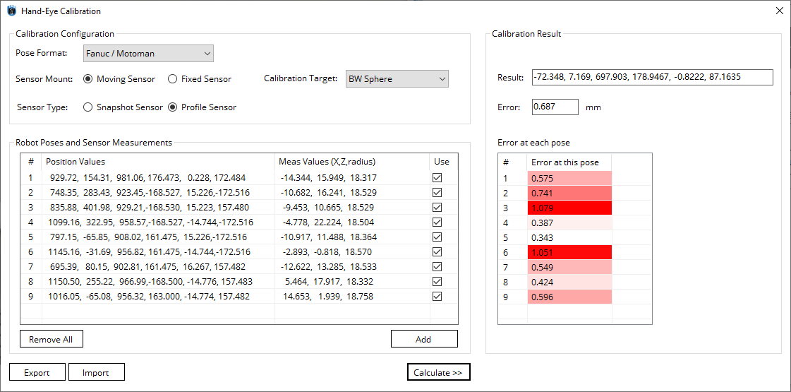
1.4.1. TCP Calibration of Fanuc with Keyence

In this example, we show the TCP calibration of FANUC M20-iA with a Keyence LJ-V7300.

Select Fanuc/Motoman in Pose Format
Select Moving Sensor in Sensor Mount and Profile Sensor in Sensor Type
Choose BW Sphere as calibration target
Program 9 robot poses to view the stationary calibration artifact from different angles. The variation between each pose is about 15 degrees.
Enter the robot pose and corresponding sensor measurement. First 6 columns represent the robot pose. The last 3 columns represent the sphere position.
Click Calculate and generate a final report. Below is an image of the result window:

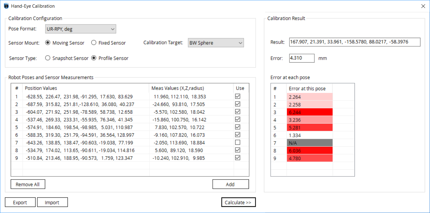
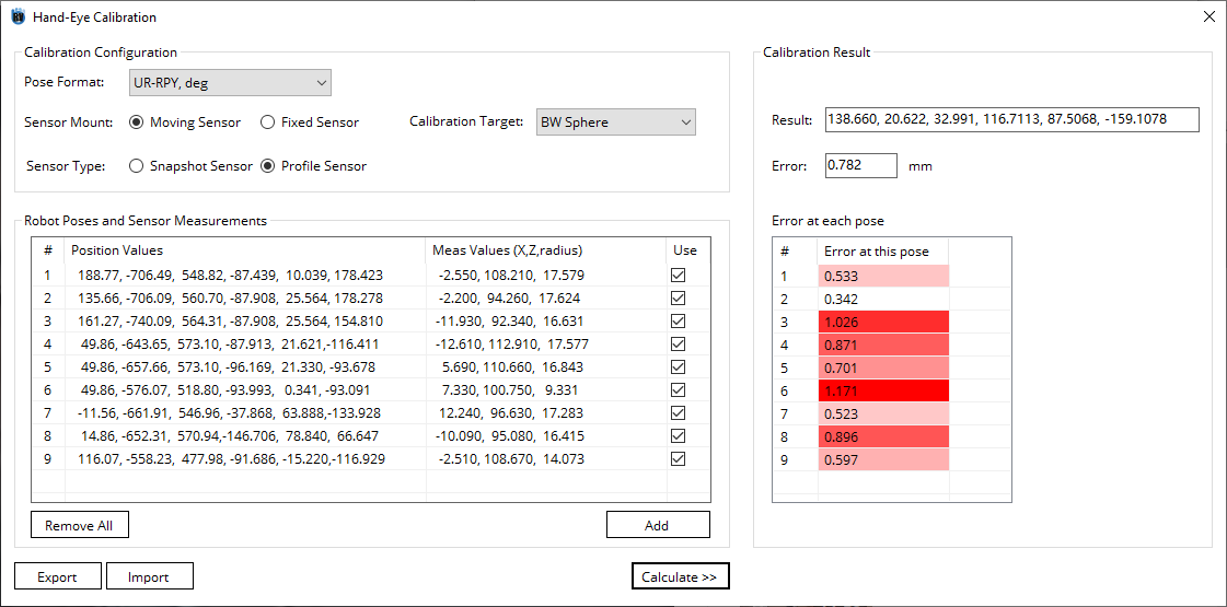
1.4.2. TCP Calibration of UR with Wenglor

In this example, we show the TCP calibration of UR 10 with a Wenglor MLSL123.

Select UR-RPY, deg in Pose Format
Select Moving Sensor in Sensor Mount and Profile Sensor in Sensor Type
Choose BW Sphere as calibration target
Program 9 robot poses to view the stationary calibration artifact from different angles. The variation between each pose is about 15 degrees.
Enter the robot pose and corresponding sensor measurement. First 6 columns represent the robot pose. The last 3 columns represent the sphere position.
Click Calculate and generate a final report. Below is an image of the result window:

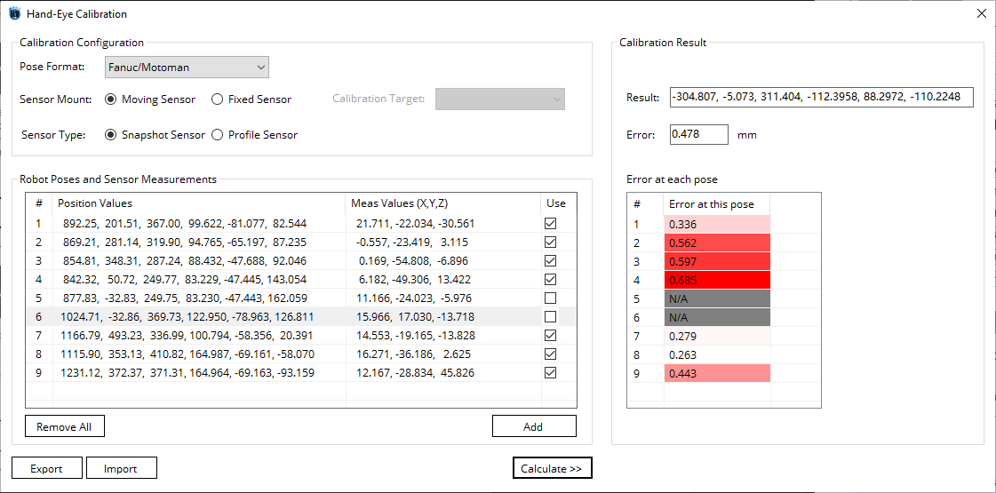
1.4.3. TCP Calibration of Fanuc with Gocator

In this example, we show the TCP calibration of FANUC M20-iA with a Gocator 3210.

Select Fanuc/Motoman in Pose Format
Select Moving Sensor in Sensor Mount and Snapshot Sensor in Sensor Type
Choose BW Sphere as calibration target
Program 9 robot poses to view the stationary calibration artifact from different angles. The variation between each pose is about 15 degrees.
Enter the robot pose and corresponding sensor measurement. First 6 columns represent the robot pose. The last 3 columns represent the sphere position.
Click Calculate and generate a final report. Below is an image of the result window:

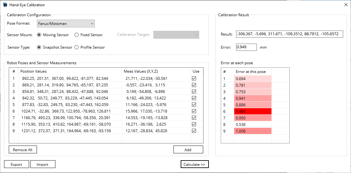
Analyze the final result. As shown in the image, pose 6 has an error over 1mm. After removing it and pose 5, the overall error is reduced to 0.478mm.

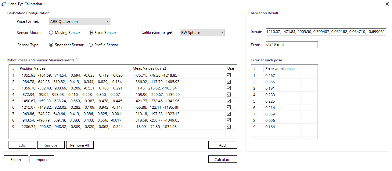
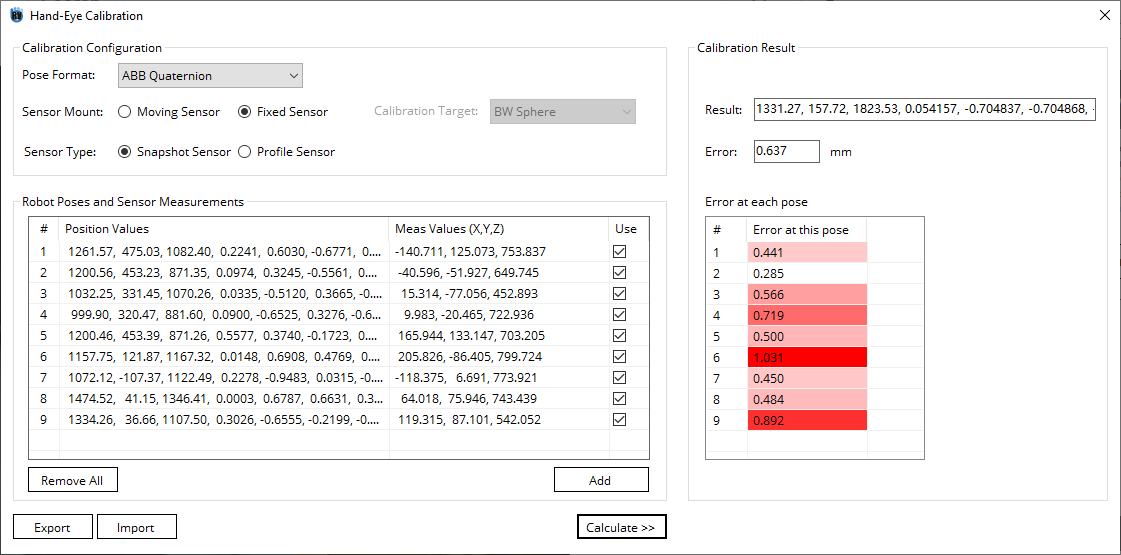
1.4.4. UF Calibration of ABB with Zivid

In this example, we show the UF calibration of ABB IRB 2600-12/1.85 with a Zivid One+ Medium. The data set could be imported from the examples.

Select ABB Quaternion in Pose Format
Select Fixed Sensor in Sensor Mount and Snapshot Sensor in Sensor Type
Choose BW Sphere as calibration target
Program 9 robot poses to view the stationary calibration artifact from different angles. The variation between each pose is about 15 degrees.
Enter the robot pose and corresponding sensor measurement. First 6 columns represent the robot pose. The last 3 columns represent the sphere position.
Click Calculate and generate a final report. Below is an image of the result window:

1.4.5. UF Calibration of Motoman with Cirrus

In this example, we show the UF calibration of Motoman GP25 with a Cirrus 300. The data set could be imported from the examples.

Select Fanuc/Motoman in Pose mode
Select Fixed Sensor in Sensor Mount and Snapshot Sensor in Sensor Type
Choose BW Sphere as calibration target
Program 9 robot poses to view the stationary calibration artifact from different angles. The variation between each pose is about 15 degrees.
Enter the robot pose and corresponding sensor measurement. First 6 columns represent the robot pose. The last 3 columns represent the sphere position.
Click Calculate and generate a final report. Below is an image of the result window:

1.4.6. TCP Calibration of Fanuc with Intel Real Sense

In this example, we show the UF calibration of Fanuc CR15iA with an Intel Real Sense.

Select Fanuc/Motoman in Pose mode
Select Moving Sensor in Sensor Mount and Snapshot Sensor in Sensor Type
Choose BW Sphere as calibration target
Program 9 robot poses to view the stationary calibration artifact from different angles. The variation between each pose is about 15 degrees.
Enter the robot pose and corresponding sensor measurement. First 6 columns represent the robot pose. The last 3 columns represent the sphere position.
Click Calculate and generate a final report. Below is an image of the result window: