2. Multi-sensor Calibration Tool

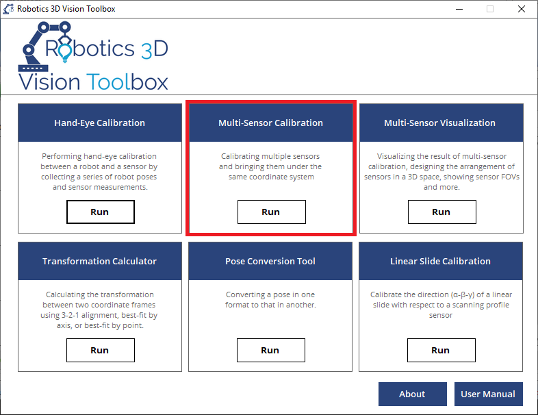
2.1. What is Multi-sensor Calibration?

Multi-sensor calibration is a process to compute the transformations between multiple vision sensors. The ability to combine the point clouds that are retrieved from different sensors allows us to scan a part that is much larger than the FOV of a single sensor. However, multi-sensor calibration is challenging because the origin of the sensor coordinate frame is not tangible. A wide variation of sensor combinations and sensor arrangements also make it difficult to use one calibration procedure that fits all sensor configurations.

To solve this issue, the toolbox provides a step-by-step wizard to help users set up multi-sensor calibration. It provides the following features:

Presets for some common multi-sensor configurations
Support for sensor type snapshot sensor/profile sensor (cannot be mixed)
Grouping sensors by whether or not they have common FOV
Support for portable CMM such as FARO tracker
Calculation of the transformation from one sensor to another sensor
Exporting the result to a .csv file
Visualization of the relative sensor position

Note

FOV: Field Of View. It refers to the area that a snapshot sensor can see, or the plane in which a profile sensor can see.

CMM: Coordinate Measuring Machine. A device that measures the geometry of physical objects by sensing discrete points on the surface of the object with a probe.

2.2. Overview

Multi-Sensor Calibration is a complex task, so we break it down to the following procedures.

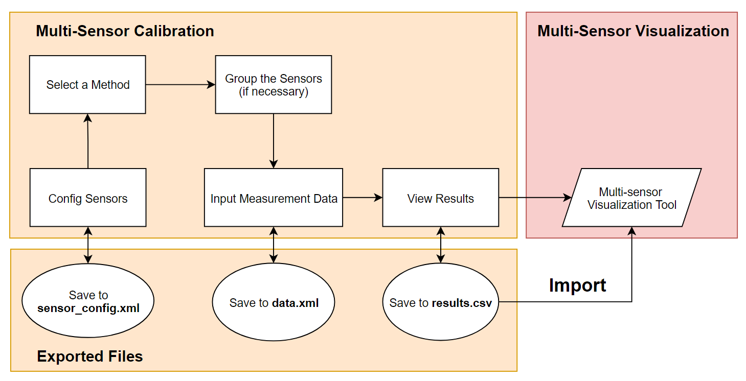
Below is a high-level overview of our Multi-Sensor Calibration Tool and Multi-Sensor Visualization Tool:
Config Sensors: Name/Brand/Model of the sensor. They are used to help select a calibration method.
Select a Method: Available methods are shown based on the sensor config.
Group the Sensors: Sensors that have a common FOV are grouped so that they can be calibrated together.
Input Measurement Data: Raw measurement values of the calibration artifact from each sensor.
View Results: View the transformation of each sensor with respect to the parent sensor.
Multi-Sensor Visualization Tool: View the relative position/orientation of the sensors in a 3D space.

The following methods are supported in the step Select a Method:
Calibration Artifact (snapshot sensor/Profile on Linear Slide): Calibrate multiple snapshot sensors with one or multiple calibration artifact.
Calibration Sphere (snapshot sensor/Profile on Linear Slide): Calibrate multiple snapshot sensors with one or multiple calibration sphere.
Calibration Sphere (profile sensor): Calibrate multiple profile sensors with one calibration sphere.
Calibration Sphere with portable CMM/Tracker (snapshot sensor): Calibrate multiple snapshot sensors with portable CMM/Tracker and one calibration sphere.
Calibration Sphere with portable CMM/Tracker (profile sensor): Calibrate multiple profile sensors with portable CMM/Tracker and one calibration sphere.
Use a large box for wide FOV snapshot sensors: Calibrate multiple snapshot sensors using a large cardboard box in the common FOV.
Use Hand-eye Calibration Results: Calibrate multiple snapshot or profile sensors with the saved TCP/UF calibration files.

Note

There are 3 files that can be exported from the Multi-Sensor Calibration Tool.

Sensor Config.xml: Name, brand, and model of each sensor. Settings regarding CMM/linear slide.
Data.xml: The raw measurement data from each sensor.
Result.csv: Transformation of each sensor with respect to the parent.

Important

Unblink3D uses X-Y-Z Euler angle (deg) format, or XYZWPR, to represent 3D transformation results between the sensors. If user requires a different format, please refer to the Pose Conversion Tool.

The following data will be used in the calibration methods:
XYZWPR: Representation of position and orientation of the calibration artifact viewed by a snapshot sensor.
XYZ: Representation of the center position of a sphere viewed by a snapshot sensor.
XZRadius: Representation of the center position of a sphere viewed by a profile sensor.

All X, Y, Z and Radius unit is mm and WPR unit is degree.

2.3. Calibration Procedure

2.3.1. Calibration Steps

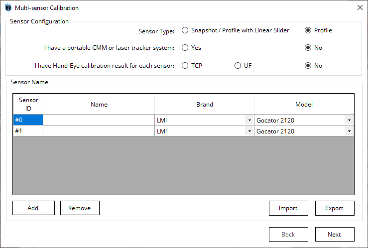
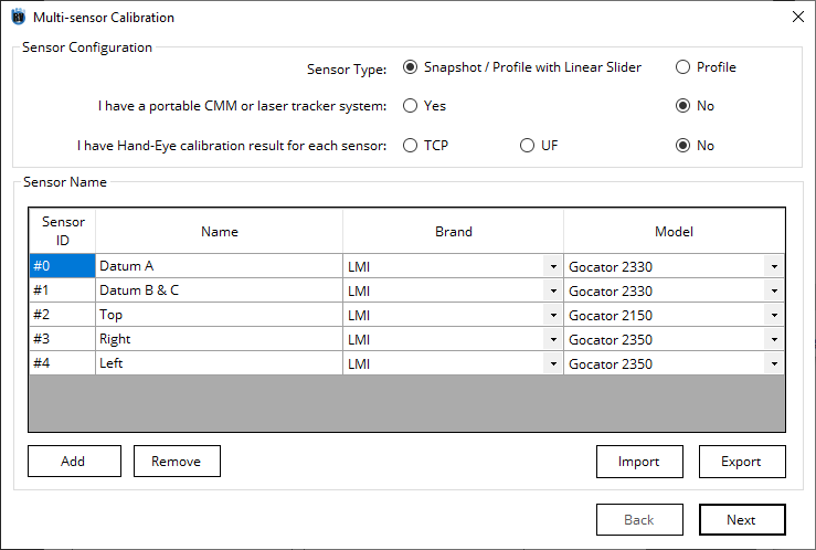
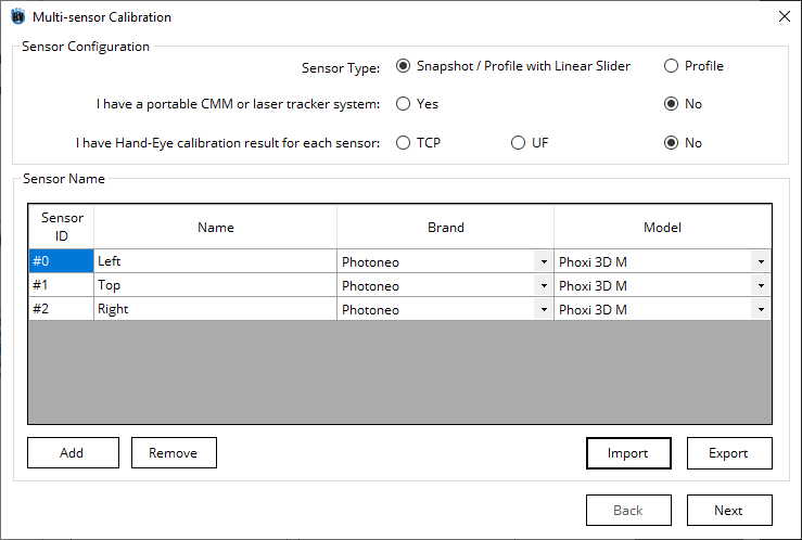
Select Snapshot or Profile from Sensor Type. A snapshot sensor can capture a point cloud (XYZ) in its FOV, while a profile sensor captures a profile (XZ) in its FOV.

Attention

When the calibration artifact is scanned by a profile sensor in motion, it needs to be treated as a snapshot sensor. Therefore the sensor type should be set as snapshot sensor.

Enter Yes or No to the answer to ” I have a portable CMM or laser tracker system “
Enter either TCP , UF or No ” I have Hand-Eye calibration result for each sensor “
Type in the name of each sensor and select the Brand and Model of the sensors, Add more sensor if required.
The Import button can be used to import a previously exported sensor configuration file. The sensor configuration can be exported for further reference by clicking on Export button. The exported file is in XML format which saves all the sensors configuration.
Click Next
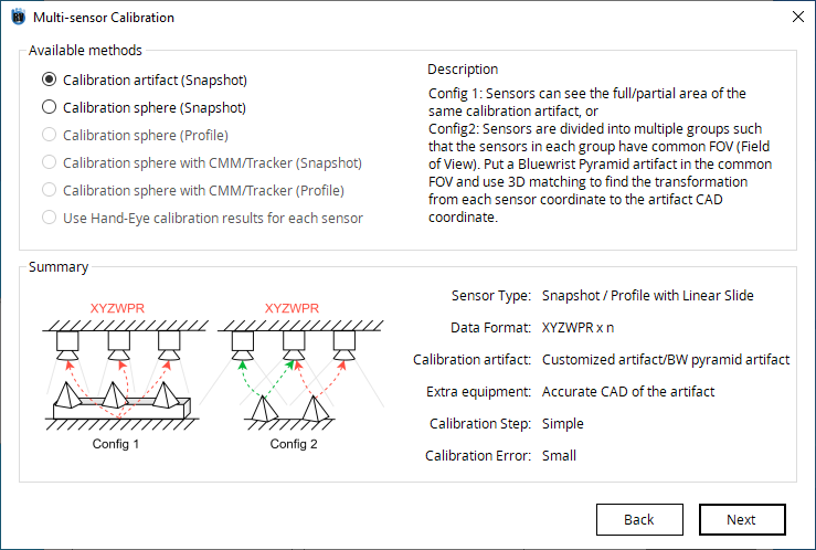
Go to Select Method tab, and choose the method available for the current setup.
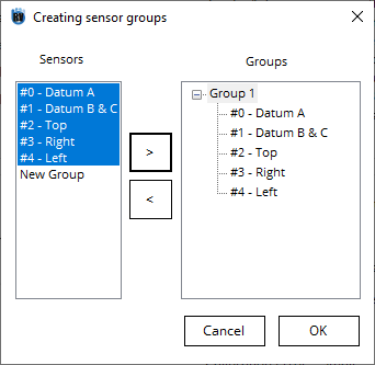
Create sensor group and assign sensors to the corresponding group by common FOV.
Select the calibration target type (if needed).
Click Compute

2.3.2. Available Methods

2.3.2.1. Calibration Artifact (snapshot sensor)

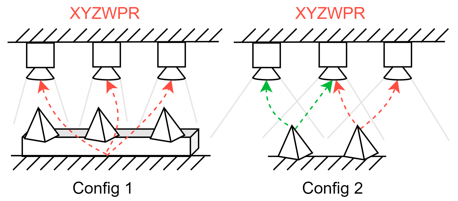
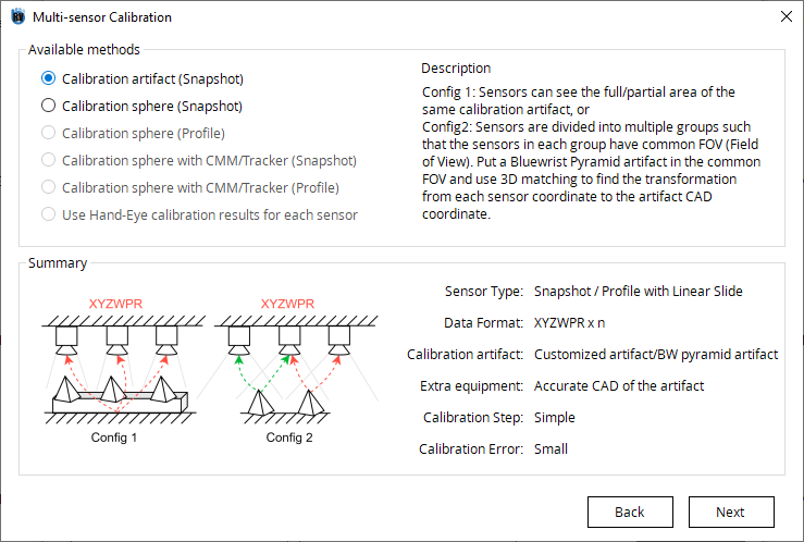
In this method, user groups the sensors such that the sensors in each group have common FOV. User uses a calibration artifact that sensors can see the full or partial area of this calibration artifact. User records the XYZWPR of the same calibration artifact in each sensor, and the toolbox computes the inter-sensor transformation.

Tip

The following components and input data are required for this method:

Calibration Artifact: BW Pyramid or Customized Calibration Artifact
Calibration File: Accurate CAD of the calibration artifact
Input Data: XYZWPR of the calibration artifact with respect to each sensor

Note

Calibration Artifact for Snapshot Sensor

BW Pyramid : A Bluewrist-made high precision solid polygon with special surface coating for high accuracy calibration.

Customized Calibration Artifact: DIY artifact by user

2.3.2.2. Calibration Sphere (snapshot sensor)

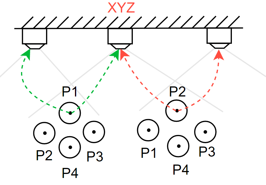
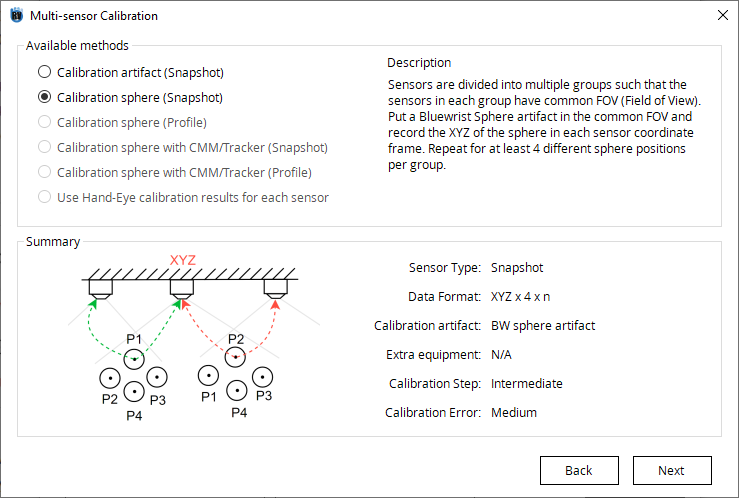
In this method, user groups the sensors such that the sensors in each group have common FOV. User records the XYZ of the same calibration sphere in each sensor, and repeat for at least 3 more new positions for each group. The toolbox computes the inter-sensor transformation.

Tip

The following components and input data are required for this method:

Calibration artifact: BW Sphere, or Customized Sphere

Input Data: XYZ of the sphere with respect to each sensor.

Note

Calibration Artifact for Profile Sensor

The calibration target should have the geometry that when the 3D sensor take its images from different orientation, the calculated target center is always the same point.

BW Sphere : A high precision sphere with special surface coating for high accuracy calibration

Customized Sphere: DIY sphere by user

2.3.2.3. Calibration Sphere (profile sensor)

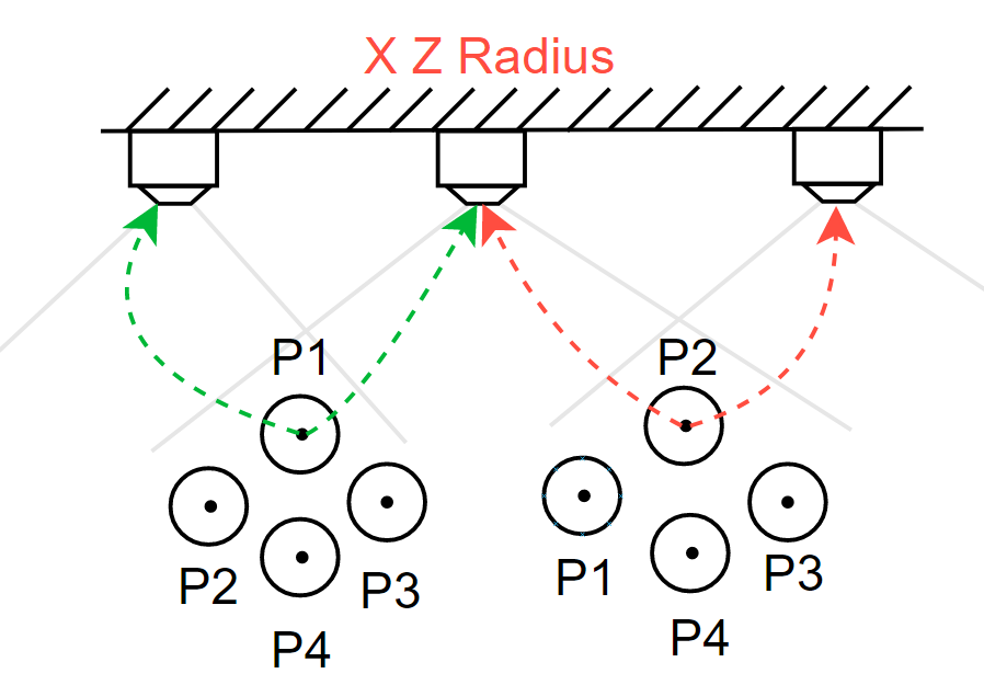
In this method, user groups the sensors such that the sensors in each group have common FOV. User records the XZRadius of the same calibration sphere in each sensor, and repeat for at least 3 more new positions for each group. The toolbox computes the inter-sensor transformation.

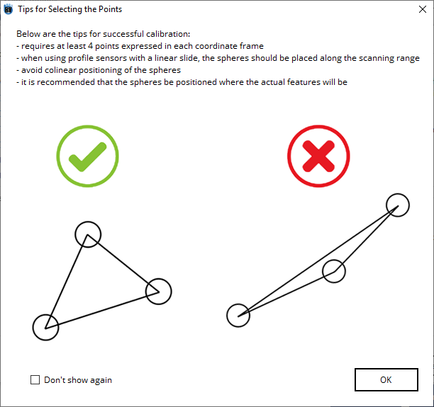
Tip

The following components and input data are required for this method:

Calibration artifact: BW Sphere, or Customized Sphere

Input Data: XZRadius of the sphere with respect to each sensor.

Note

XZRadius : X, Z, Radius is calculated from the circle which the profile sensor plane intersects with the sphere. X and Z is the center of the circle.

2.3.2.4. Calibration sphere with CMM/Tracker (snapshot sensor)

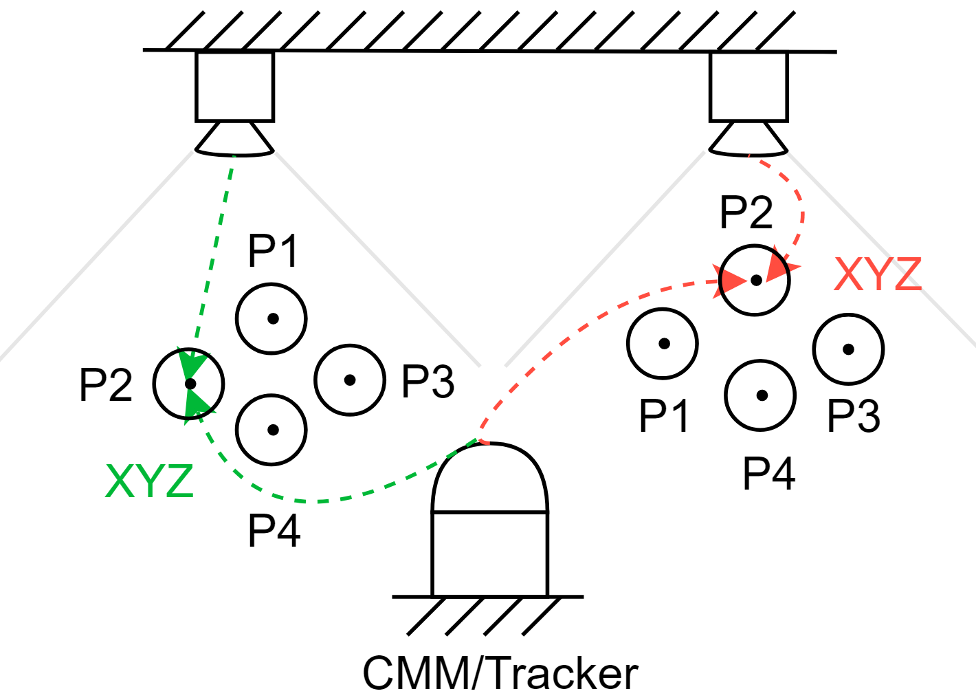
In this method, thanks to the high accuracy of the portable CMM/Tracker, the user can calibrate sensors that are far away from each other. The user records the XYZ of a calibration sphere in each sensor and in the portable CMM/Tracker coordinate, and repeat for at least 3 more new positions for each sensor. This helps associates the sensor coordinate to the portable CMM/Tracker coordinate. Then the toolbox computes the inter-sensor transformation.

Tip

The following components and input data are required for this method:

Calibration artifact: BW Sphere, or Customized Sphere
External measurement device: portable CMM or Laser Tracker
Input Data: XYZ of one sphere with respect to each sensor and the portable CMM coordinate frame. Move the sphere and repeat for at least 3 more new positions.

2.3.2.5. Calibration sphere with CMM/Tracker (profile sensor)

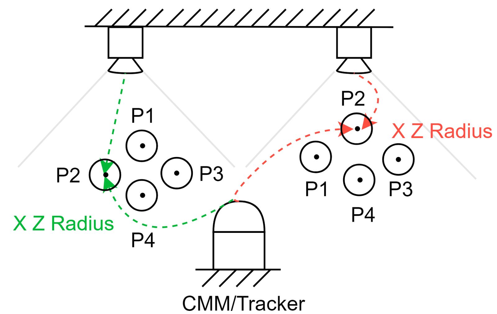
In this method, thanks to the high accuracy of the portable CMM/Tracker, the user can calibrate sensors that are far away from each other. The user records the XZRadius of a calibration sphere in each sensor and in the portable CMM/Tracker coordinate, and repeat for at least 3 more new positions for each sensor. This helps associates the sensor coordinate to the portable CMM/Tracker coordinate. Then the toolbox computes the inter-sensor transformation.

Tip

The following components and input data are required for this method:

Calibration artifact: BW Sphere, or Customized Sphere
External measurement device: portable CMM
Input Data: XZRadius of one sphere with respect to each sensor and the portable CMM coordinate frame. Move the sphere and repeat for at least 3 more new positions.

2.3.2.6. Use a large box for wide FOV snapshot sensors

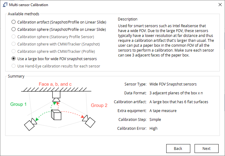
Many modern smart sensors that have large FOV (e.g. Intel Realsense) are not suitable for calibration using spheres or pyramid artifacts because the depth resolution decreases significantly as the distance increases. Fortunately, these applications do not typically require an accuracy of sub-millimeter level and thus can be calibrated using some other artifacts that are readily avaialble.

In this method, users can calibrate sensors that are far away from each other using large cardboard boxes. The user needs to label the cardboard box properly beforehand, take the snapshot in each camera, and extract the planes. The toolbox will compute the sensor-to-sensor transformation using the information provided.

Tip

The following components and input data are required for this method:

Calibration artifact: a cardboard box
External measurement device: a tape measure
Input Data: Box UF in the format of XYZWPR

2.3.2.7. Use Hand-eye Calibration Results

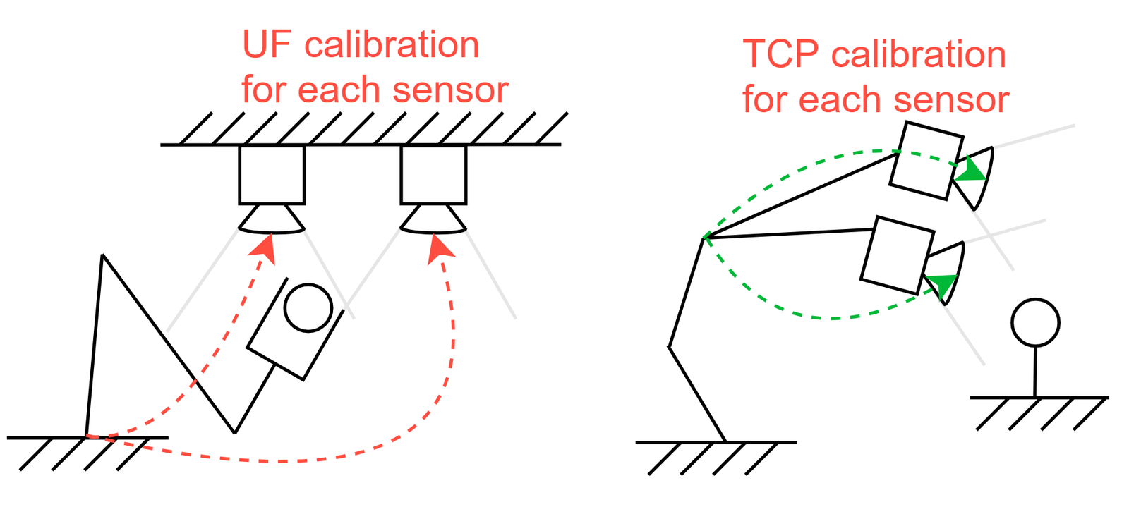
In this method, user directly import the TCP/UF calibration result that was obtained using the Hand-Eye Calibration Toolbox. The calibration result is saved in .xml format, which associates the sensor coordinate with the robot base/flange. The toolbox computes the inter-sensor transformation.

Tip

The following components and input data are required for this method:

Input Data: XYZWPR of one vision sensor to the robot base/flange

2.3.3. Sensor Measurement Collection

After a method is selected, click Next. If a previous sensor configuration is imported, a pop up message will give user the option to import the past saved sensor data. If the user prefers collecting new data, then he/she needs to create sensor groups. The sensors which have the same FOV should be put into the same group.

For snapshot and profile sensor data collection, please refer to Section 1.3.2.

2.3.4. Calibration Result Review

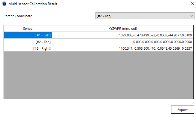
In the result window, user can select a parent sensor and display the transformation to all other sensors. User can also select the calibration artifact as the parent coordinate frame.

Click Export button and save the final result in a .csv file.

2.4. Examples

Here, we present some step-by-step examples on how our industrial partners use the multi-sensor calibration toolbox.

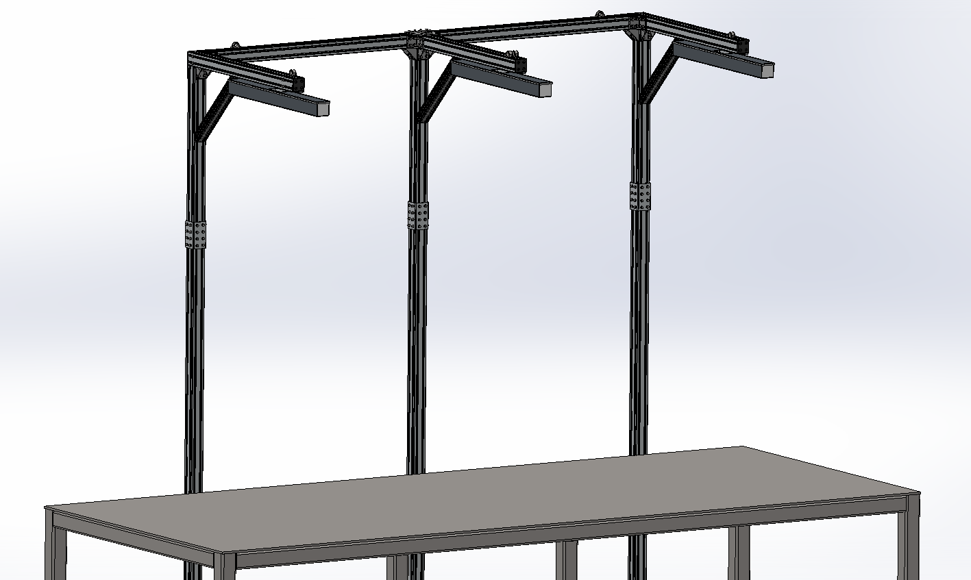
2.4.1. 5 profile sensors with a linear slide to scan a big part

In this project, it is required to perform a multi-sensor calibration for 5 stationary profile sensors. The part was placed on a linear slide and was scanned by the profile sensors that surround it.

Sensor Name	Model Name
Datum A	LMI Gocator 2330
Datum B & C	LMI Gocator 2330
Top	LMI Gocator 2150
Right	LMI Gocator 2350
Left	LMI Gocator 2350

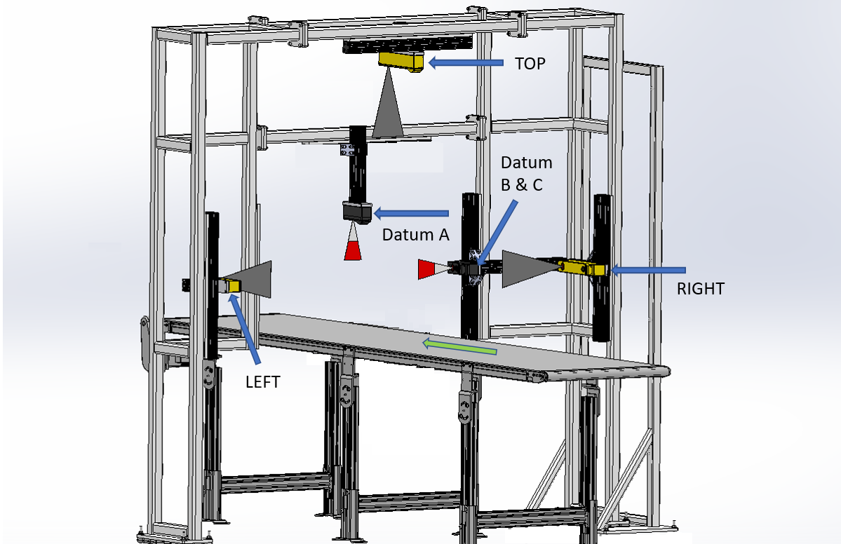
The sensors don’t have common FOV, so a customized calibration artifact is built. It’s designed in a way that each sensor can see a BW pyramid and a BW sphere in its FOV when the artifact moves along the linear slide.

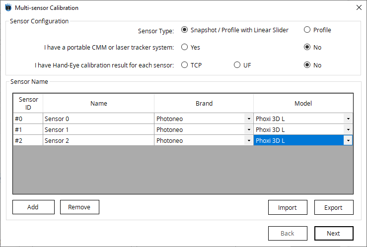
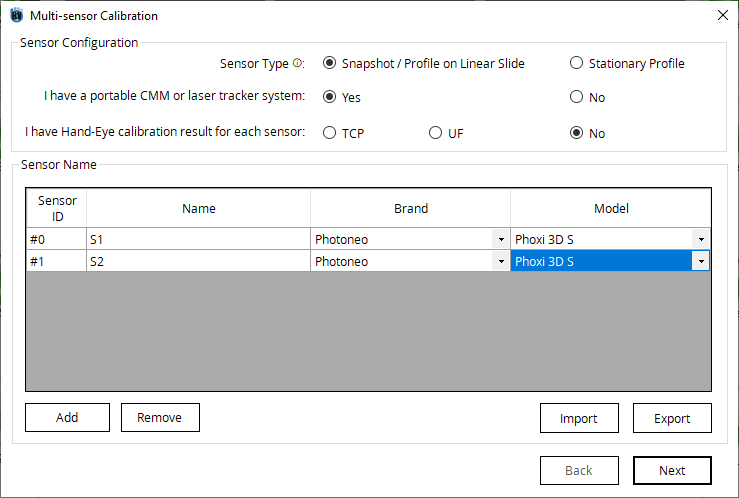
Open the toolbox and select Multi-sensor Calibration. Enter Sensor Type and fill out if there is portable CMM and Hand-Eye calibration result. Type in the name of each sensor and select the Brand and Model of sensors.

Go to Available Methods tab, and there are two methods available for the current setup. Select Calibration artifact (Snapshot) and click Next.

The sensors need to be grouped by whether or not they look at the same calibration artifact. In this example, all sensors are looking at the same CAD so put all sensors under Group1.

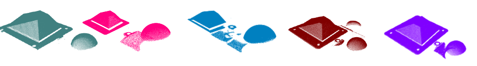
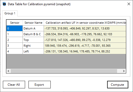
Below are the point clouds generated from each sensor. By matching the point cloud with the CAD model, user obtain the XYZWPR of the CAD model with respect to each sensor coordinate frame.

Sensor	Calibration artifact UF in the sensor coordinate frame X,Y,Z,W,P,R (mm, deg)
Datum A	-137.733, 318.093, -406.849, 92.297, 8.521, 13.630
Datum B & C	-266.534, 304.316, -66.903, -178.295, 76.662, 92.103
Top	-127.810, 147.326, -480.890, 89.275, -0.338, 12.279
Right	189.940, 159.474, -296.619, -4.717, -78.001, 93.365
Left	-206.131, 138.340, 16.946, 178.485, 78.714, 88.252

Group 1: All sensors

Calibration Artifact: Customized Calibration Artifact

Note

The toolbox only supports the BW pyramid 3D matching at the moment.

Type in the XYZWPR of the calibration artifact in each sensor coordinate frame. In other words, type in the transformation from the sensor coordinate frame to the CAD coordinate frame. Click Compute.

Tip

User can Right Click on the cells to Copy or Paste the data to Excel.

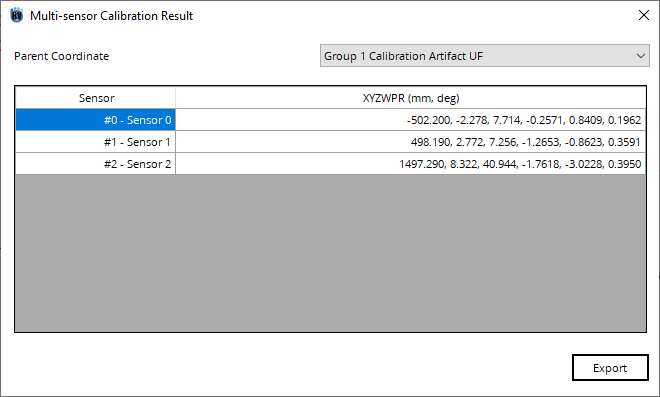
In the result window, users can select a parent sensor and display the transformation to all other sensors. Click Export button and save the final result in a .csv file.

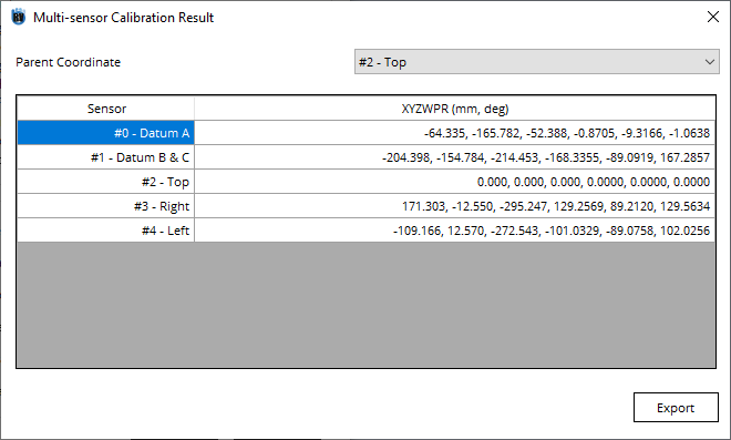
Note

Choose the parent coordinate before clicking the Export button. User can also select the calibration artifact as the parent coordinate frame.

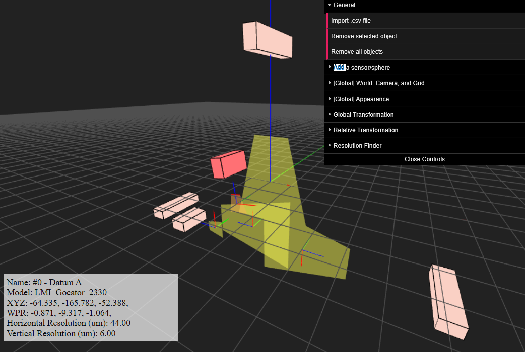
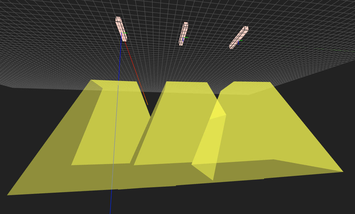
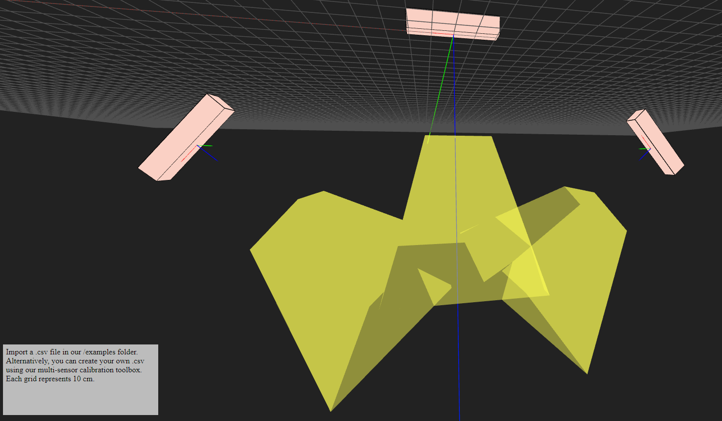
A 3D visualization tool also pops up after exporting the result to .csv. By importing the .csv file, the user can see the positions/size/FOV of the sensors in a 3D space. For more information about the visualization tool, refer to Multi-Sensor Visualization Tool.

2.4.2. 3 stationary snapshot sensors with a pyramid target

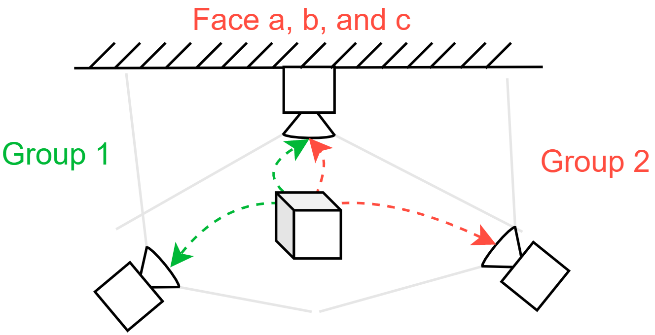
In this project, it is required to perform a multi-sensor calibration for three stationary snapshot sensors. Only adjacent sensors have common FOV, so the sensors are divided into 2 groups and a calibration artifact is placed in the common FOV of each group.

Sensor Name	Model Name
Sensor 0	Photoneo Phoxi 3D L
Sensor 1	Photoneo Phoxi 3D L
Sensor 2	Photoneo Phoxi 3D L

Open the toolbox and select Multi-sensor Calibration. Enter Sensor Type and fill out if there is portable CMM and Hand-Eye calibration result

Go to Available Methods tab, and there are two methods available for the current setup. Select Calibration artifact (Snapshot) and click Next.

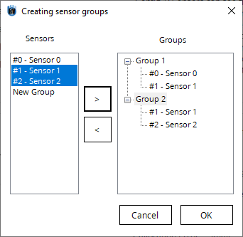
Put Sensor 0 and Sensor 1 under Group 1 because they have common FOV and thus they look at the same calibration artifact. Similarly, put Sensor 1 and Sensor 2 under Group 2.

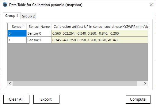
By matching the point cloud with the CAD model, user obtain the XYZWPR of the CAD model with respect to each sensor coordinate frame.

Group 1

Sensor	Calibration artifact UF in the sensor coordinate frame X,Y,Z,W,P,R (mm, deg)
Sensor 0	0.560, 502.264, -0.340, 0.260, -0.840, -0.200
Sensor 1	0.345, -498.250, 0.250, 1.260, 0.870, -0.340

Group 2

Sensor	Calibration artifact UF in the sensor coordinate frame X,Y,Z,W,P,R (mm, deg)
Sensor 1	-0.450, 499.560, 0.960, -0.320, -1.200, 1.180
Sensor 2	0.560, -500.260, 1.200, 0.220, 0.950, 1.200

Group 1: Sensor 0 and Sensor 1
Group 2: Sensor 1 and Sensor 2
Calibration Artifact: BW Pyramid Artifact

Type in the XYZWPR of the calibration artifact in each sensor coordinate frame. In other words, type in the transformation from the sensor coordinate frame to the CAD coordinate frame. Click Compute.

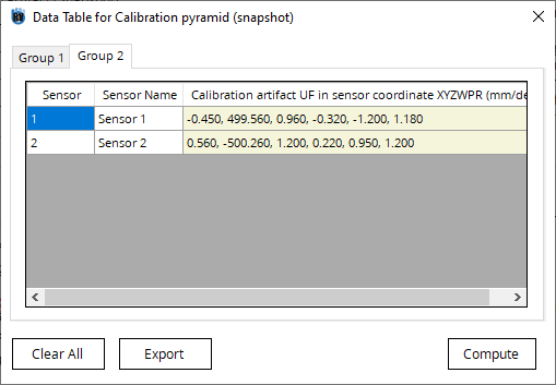
In the result window, users can select a parent sensor and display the transformation to all other sensors. Click Export button and save the final result in a .csv file.

Note

Choose the parent coordinate before clicking the Export button. You can also select the calibration artifact as the parent coordinate frame.

A 3D visualization tool also pops up after exporting the result to .csv. By importing the .csv file, the user can see the positions/size/FOV of the sensors in a 3D space. For more information about the visualization tool, refer to Multi-Sensor Visualization Tool.

2.4.3. 3 stationary snapshot sensors with a sphere target

In this project, it is required to perform a multi-sensor calibration for three stationary snapshot sensors. Only adjacent sensors have common FOV, and the FOV is large that the BW pyramid calibration artifact cannot generate a accurate result. User decided to divide them into 2 groups and place a calibration sphere in the common FOV of each group.

Sensor Name	Model Name
Left	Photoneo Phoxi 3D M
Top	Photoneo Phoxi 3D M
Right	Photoneo Phoxi 3D M

Group 1: Sensor #1 Left and Sensor #2 Top
Group 2: Sensor #2 Top and Sensor #3 Right
Calibration Artifact: BW Sphere Artifact

Note

Whether to use a BW Pyramid or BW Sphere as the calibration target depends on the sensor configuration and user needs.

In general, using a pyramid requires less measurements but requires point cloud matching. It also requires a larger calibration target if the FOV is larger. On the other hand, using a calibration sphere requires more measurements and does not requires point cloud matching.

If the common FOV is large, using sphere artifacts often gives a better result than a BW pyramid, given that they are positioned properly.

Enter Sensor Type and fill out if there is portable CMM and Hand-Eye calibration result

Go to Available Methods tab, and you can see that two methods are available for the current setup. Select Calibration sphere (snapshot) and click Next.

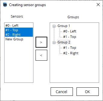
In the sensor group config window, select Sensor #1 on the left and click Add >> to add the sensor to Group 1. Alternatively, you can Double Click to add a sensor to the selected group. Also add Sensor #2 to Group 1.

Select New Group on the left and click Add >> to create a new group. Add Sensor #2 and Sensor #3 to Group 2.

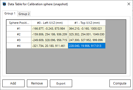
A form will be generated based on the sensor group config.

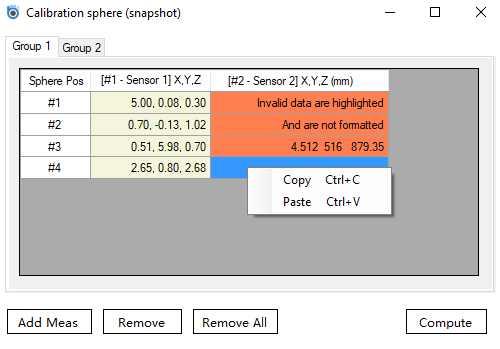
In Group 1, put the calibration sphere in the common FOV of Sensor #1 and Sensor #2. Record the position of the sphere in both sensors in XYZ format in row Pos #1.

Click Add Meas to create a new row. Move the sphere to the second position and record the XYZ in row Pos #2. Repeat for Pos #3 and Pos #4.

Group 1

Sphere Pos	Sensor #1 Left X,Y,Z (mm)	Sensor #2 Top X,Y,Z (mm)
Position 1	-166.877, -0.243, 873.984	364.210, -0.16, 1000.021
Position 2	-159.806, 254.186, 936.209	325.302, 254.001, 1049.030
Position 3	-249.609, 328.096, 956.715	247.300, 327.952, 999.896
Position 4	-321.734, 20.180, 911.461	228.040, 19.906, 917.013

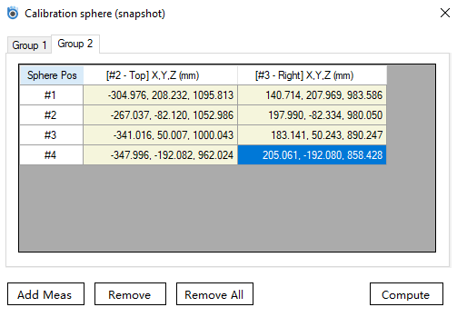
Group 2

Sphere Pos	Sensor #2 Top X,Y,Z (mm)	Sensor #3 Right X,Y,Z (mm)
Position 1	-304.976, 208.232, 1095.813	140.714, 207.969, 983.586
Position 2	-267.037, -82.120, 1052.986	197.990, -82.334, 980.050
Position 3	-341.016, 50.007, 1000.043	183.141, 50.243, 890.247
Position 4	-347.996, -192.082, 962.024	205.061, -192.080, 858.428

Note

A minimum of 4 positions are required.

Warning

The positions of the calibration sphere is not arbitrary. In order for the algorithm to calculate the transformation between the sensors, the 4 points should not be in the same plane. Ideally the vectors formed should be as linearly independent as possible.

The table has auto validation feature that helps check the user input. If the data are valid, the cell turns green and the data are formatted. If the data are invalid, it turns yellow and the data are not formatted. In addition, the user can right click on the cell to copy and paste data directly from MS Excel.

Click Compute and show the calibration error between each pair of sensors.

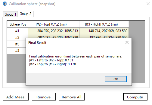
If user is satisfied with the result and do not need to collect any more data, user can view the final result in the result window.

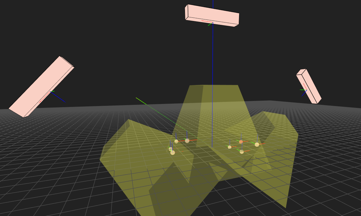
A 3D visualization tool also pops up after exporting the result to .csv. By importing the .csv file, the user can see the positions/size/FOV of the sensors in a 3D space. For more information about the visualization tool, refer to Multi-Sensor Visualization Tool.

2.4.4. 3 stationary profile sensors with a sphere target

In this project, user wants to perform a multi-sensor calibration for three stationary profile sensors. Only adjacent sensors have common FOV, so the sensors are divided into 2 groups. User places a sphere artifact in the common FOV of each group, recording the X, Z, and radius of the profile in each sensor coordinate.

Sensor Name	Model Name
Left	LMI Gocator 2375
Top	LMI Gocator 2375
Right	LMI Gocator 2375

Group 1: Sensor #0 Left and Sensor #1 Top
Group 2: Sensor #1 Top and Sensor #2 Right
Calibration Artifact: BW Sphere Artifact

Note

When performing multi-sensor calibration of profile sensors, a sphere artifact that has a larger diameter helps reduce the error.

Enter Sensor Type and fill out if there is portable CMM and Hand-Eye calibration result

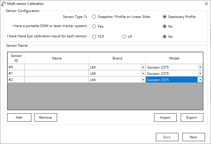
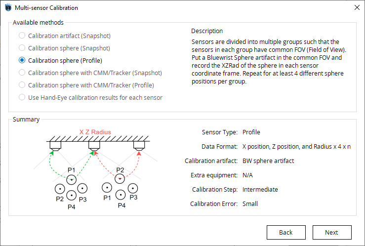
Go to Available methods section, and you can see that one method is available for the current setup. Select Calibration sphere(Profile) and click Next.

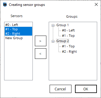
In the sensor group config window, select Sensor #0 (Left) on the left and click Add >> to add the sensor to Group 1. Alternatively, you can Double Click to add a sensor to the selected group. Also add Sensor #1 (Top) to Group 1.

Select New Group on the left and click Add >> to create a new group. Add Sensor #1 (Top) and Sensor #2 (Right) to Group 2.

When OK is selected a couple tips will be presented.

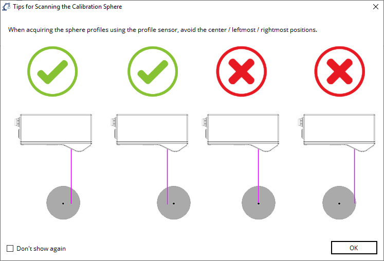
A new window will be presented based on the sensor group config. Here is where the profile data will be entered for calculations.

Note

Because 2 Groups were created earlier in the example, only 2 groups will be available.

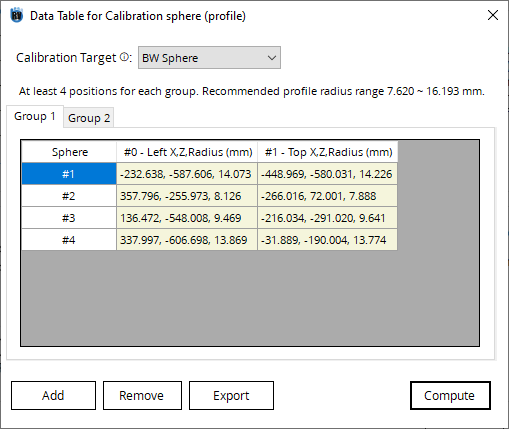
In Group 1, the user needs to place the calibration sphere in the common FOV of the 2 sensors in the group (Left and Top).

Record the X, Z, and radius of the sphere for both sensors.

The user must make sure that when measuring the sphere, that the radius of the sphere falls between the valid range specified. The range is calculated based on the nominal diameter of the sphere in this case, for the BW Sphere the range is 7.620 ~ 16.913 mm.

Note

If A Customised Sphere is selected, the recommended profile radius range will change when the Diameter is entered.

Group 1:

Sphere Pos	Sensor #1 (Left) X,Z,rad (mm)	Sensor #2 (Top) X,Z,rad (mm)
Position 1	-232.638, -587.606, 14.073	-448.969, -580.031, 14.226
Position 2	357.796, -255.973, 8.126	-266.016, 72.001, 7.888
Position 3	136.472, -548.008, 9.469	-216.034, -291.02, 9.641
Position 4	337.997, -606.698, 13.869	-31.889, -190.004, 13.774

Click Add to create a new row. Move the sphere to the second position and record the X,Z,rad in row Pos #2. Repeat for Pos #3 and Pos #4.

Note

A minimum of 4 positions are required.

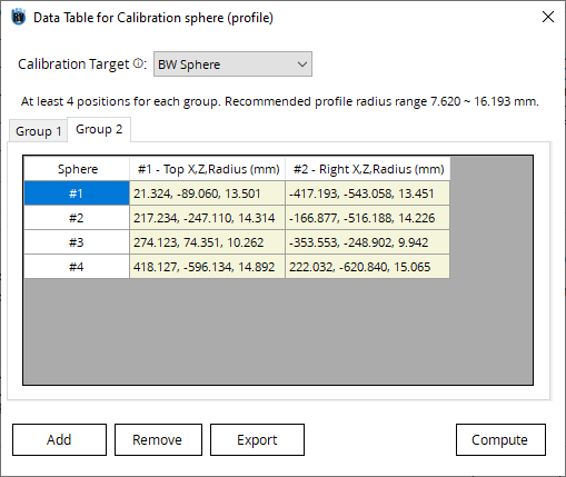
Repeat the same procedure for Group 2.

Group 2

Sphere Pos	Sensor #2 (Top) X,Z,rad (mm)	Sensor #3 (Right) X,Z,rad (mm)
Position 1	21.324, -89.06, 13.501	-417.193, -543.058, 13.451
Position 2	217.234, -247.11, 14.314	-166.877, -516.188, 14.226
Position 3	274.123, 74.351, 10.262	-353.553, -248.902, 9.942
Position 4	418.127, -596.134, 14.892	222.032, -620.84, 15.065

Note

When recording the X,Z,rad, it isn’t needed to specify the side on which the spheres are at with respect to the sensor coordinate frame because the toolbox iterates through all combinations of signs and picks the one that has smallest error.

Warning

When the radius (or rad) is too small or too big, the cell turns yellow. Technically, the value is still valid; however, it may results in larger error and thus is not allowed.

Click Compute. According to the actual setup, select Yes or No to decide the relative positions of each pair of sensors.

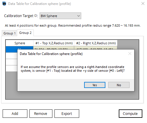
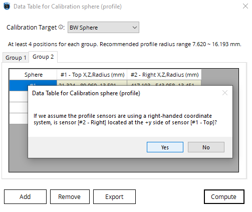
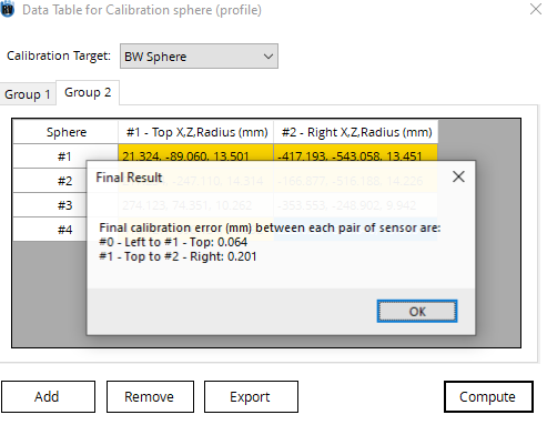
Note

Since there are always a pair of configurations (see below) that generates the same amount of error, the user has to pick up one of them.
In our toolbox, this is done by looking at the sign of Y that is based on a right-handed coordinate system.
(1) X, Y, Z, W, P, R
(2) X, -Y, Z, -W, P, -R

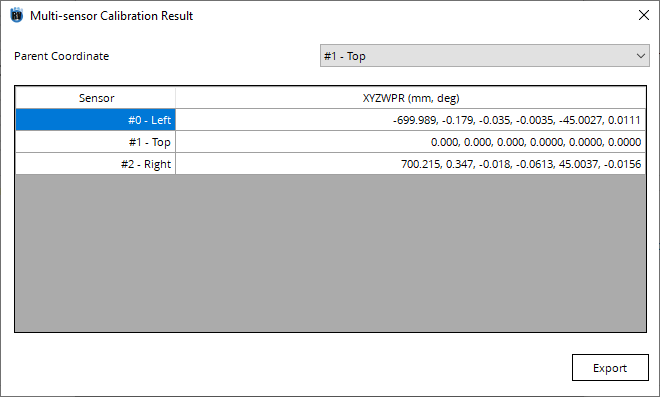
In the end, the result window shows the calibration error between each pair of sensors.

If user is satisfied with the result and do not need to collect any more data, user can view the final result in the result window, or in the 3D visualization tool.

A 3D visualization tool also pops up after exporting the result to .csv. By importing the .csv file, the user can see the positions/size/FOV of the sensors in a 3D space. For more information about the visualization tool, refer to Multi-Sensor Visualization Tool.

2.4.5. 2 profile sensors mounted on a linear slide: α-β-γ calibration and multi-sensor calibration using 4 spheres

In this project, 2 profile sensors that have a common FOV are mounted on a linear slide. The sensors are triggered using the encoder of the linear slide, and we want to get the point clouds of the parts by combining the two point clouds from the two sensors.

Therefore, first we need to perform an α-β-γ calibration for each sensor so that the point cloud from both sensors are not deformed. Second, we need to do a multi-sensor calibration so that the point clouds from the buddy sensor can be brought to the parent sensor coordinate frame.

Sensor Name	Model Name
Parent	LMI GoCator 2330
Buddy	LMI GoCator 2330

At the moment, out Robotic 3D Vision Toolbox doesn’t provide α-β-γ calibration feature (currently under development), so the user needs to compute the α-β-γ of each sensor using third-party software. The α-β-γ calibration results are as follows:

α-β-γ calibration result

Sensor	α-β-γ calibration result (deg)
Parent	88.812, 1.481, 89.115
Buddy	89.500, 4.350, 94.321

Configure the profile sensor properly using the α-β-γ values so that they can generate a point cloud that reflects the true shape of the scanned part.

Open the toolbox and select Multi-sensor Calibration. Enter Sensor Type and fill out if there is portable CMM and Hand-Eye calibration result

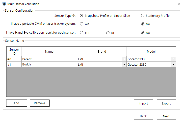
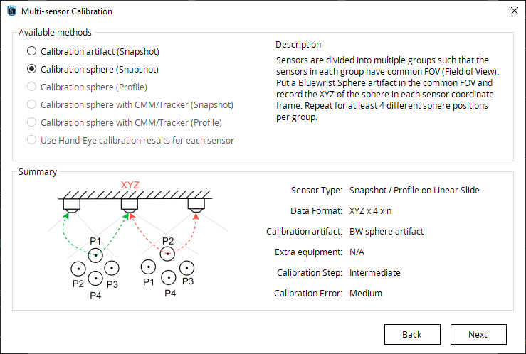
Go to Available Method section, and there are two methods available for the current setup. Select Calibration sphere (Snapshot) and click Next.

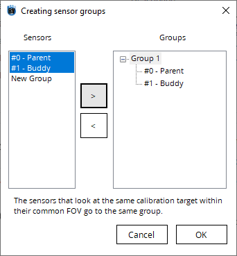
Put Parent Sensor and Buddy Sensor under Group 1 because they have common FOV and thus they look at the same calibration artifact.

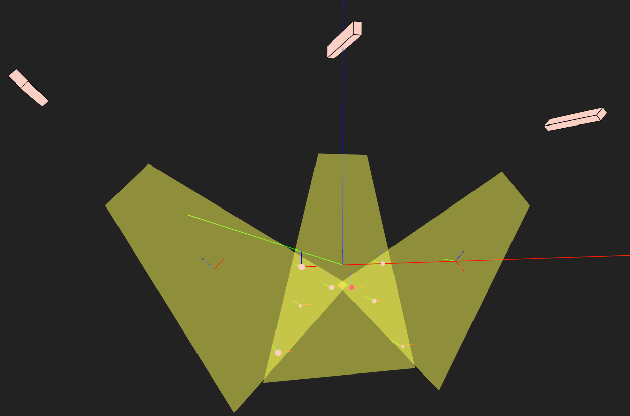
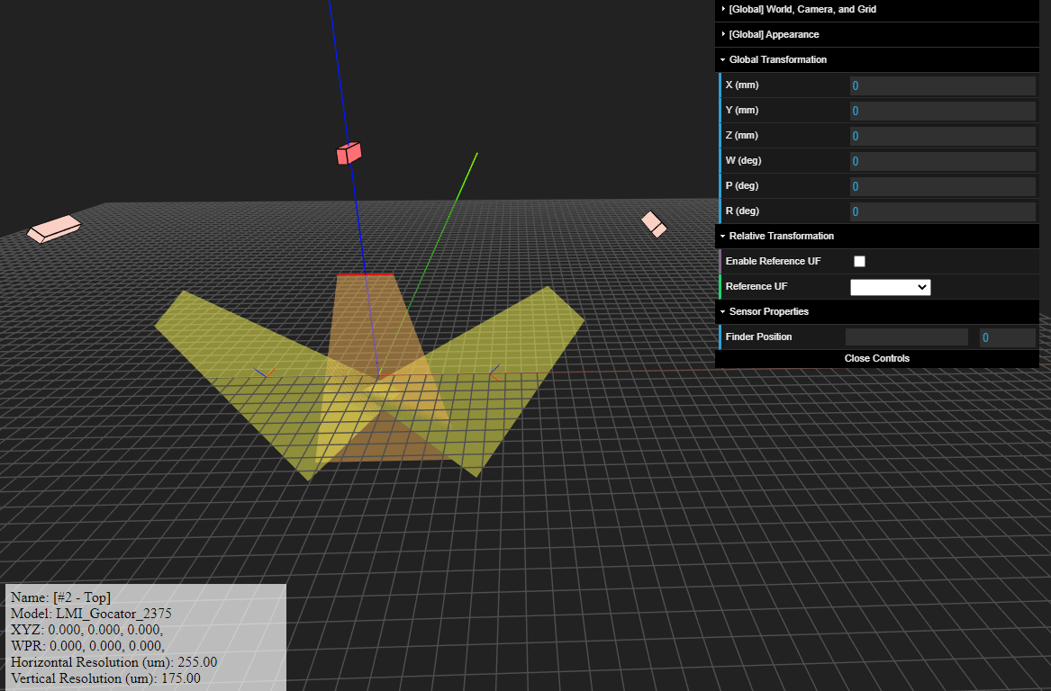
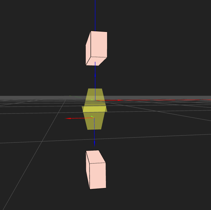
For multi-sensor calibration, we need to know the position of the same spheres expressed in Parent Sensor and Buddy Sensor, respectively. The image below shows the point cloud generated from the two sensors, but expressed in its own coordinate frame.

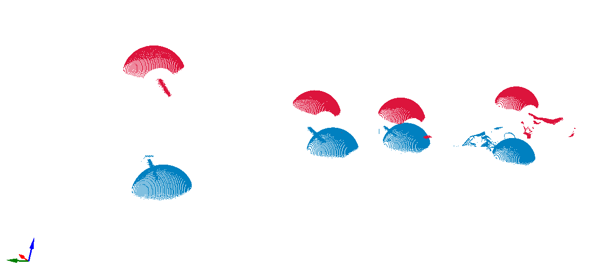
Warning

The positions of the calibration sphere is not arbitrary. In order for the algorithm to calculate the transformation between the sensors, the 4 points should not be in the same plane. Ideally the vectors formed should be as linearly independent as possible. Try to put them at different x, y, and z, and not to put them along the same line.

For extracting the center of the sphere, you can either use third-party point cloud processing software, or our built-in PCL viewer. If you want to use our built-in PCL viewer, select a cell and click Load PCL button.

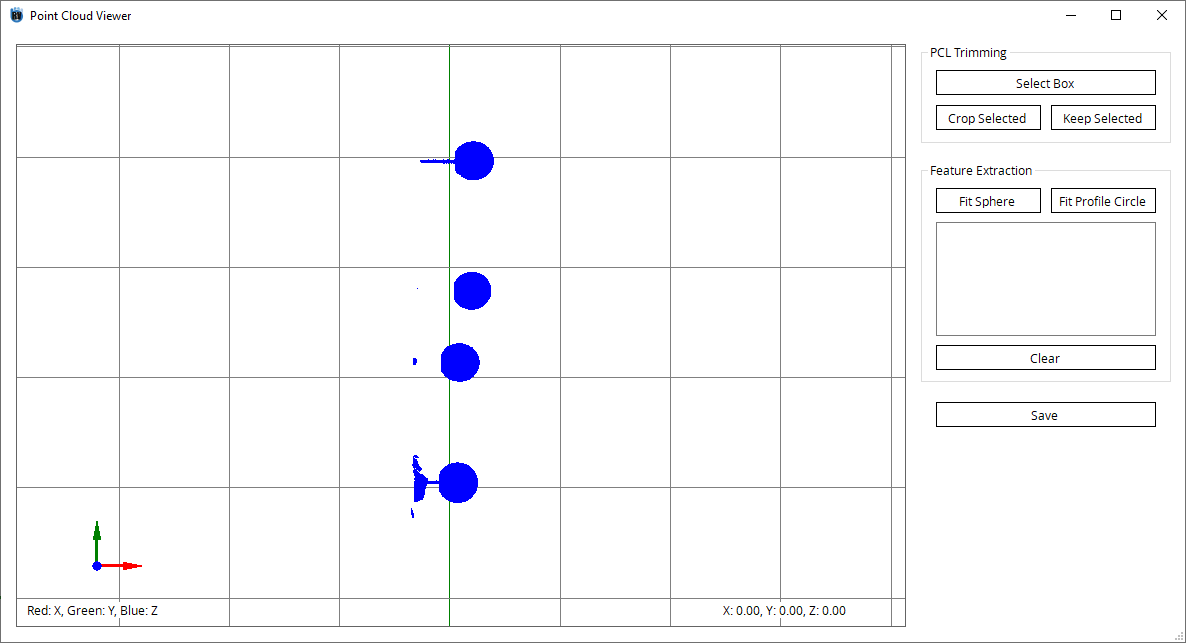
In the PCL viewer, remove the unwanted point cloud and perform the sphere extraction.

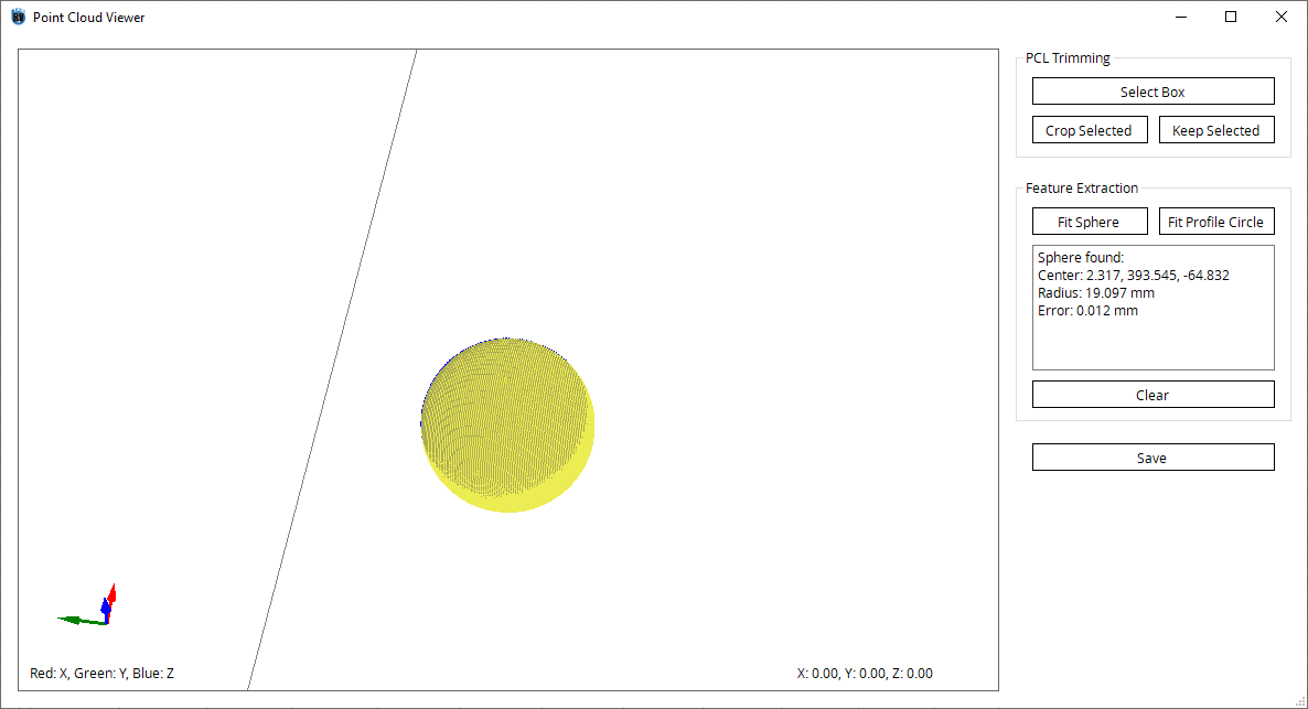
Repeat for all the spheres can click Compute.

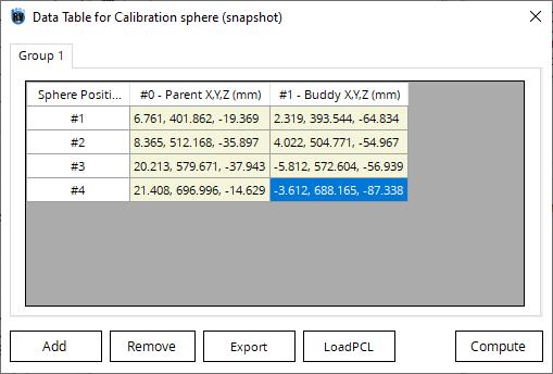
Finally, we get the relationship between the two sensors.

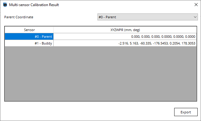
You can use the built-in 3D Visualization Tool to view the result.

2.4.6. 2 stationary snapshot sensors with a CMM

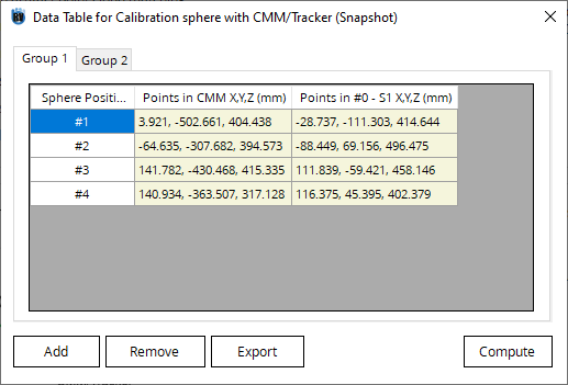
In this project, the user wanted to perform a multi-sensor calibration for two stationary snapshot sensors. The sensors don’t have common FOV, so the user decided to use a CMM to calibrate the sensors. Four spheres were placed in the FOV of each sensor, and the position of each sphere with respect to the CMM is recorded.

The image below shows the configuration of the sensors and the spheres.

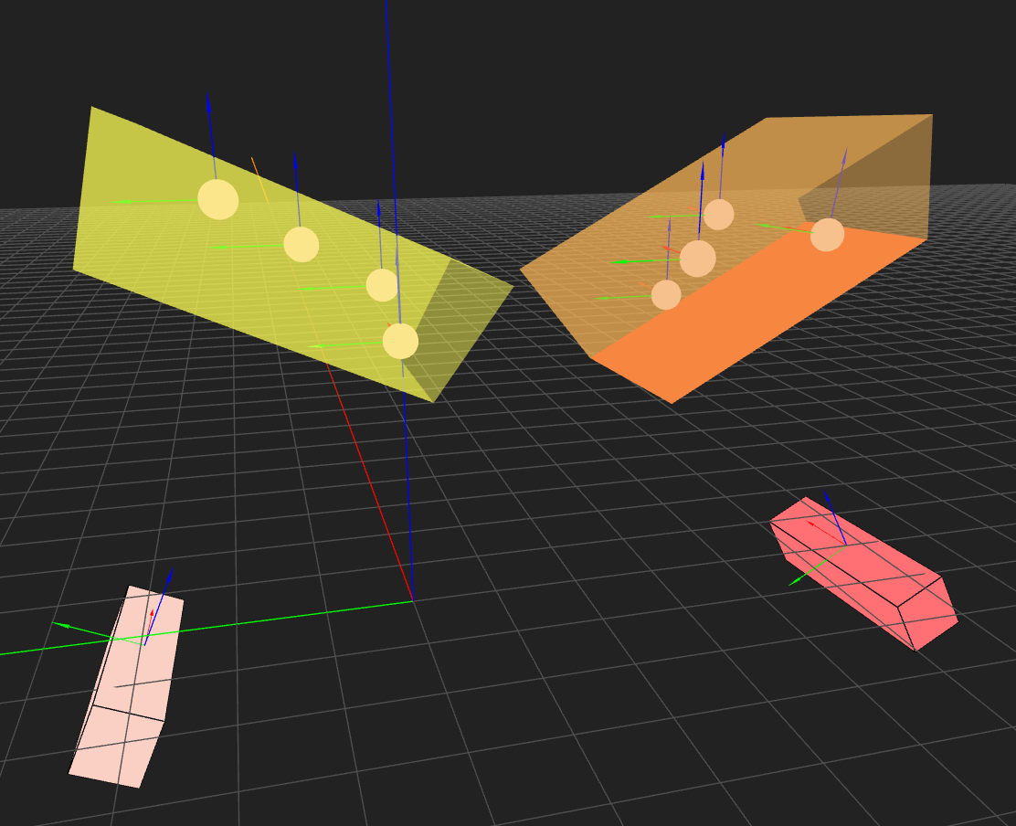
Below are the data collected.

Sensor Name	Model Name
S1	Photoneo Phoxi 3D S
S2	Photoneo Phoxi 3D S

Sphere Name	Sphere Position in CMM (mm)	Sphere Position in Sensor Coordinate (mm)
S1-1 (in S1)	3.921, -502.661, 404.438	-28.737, -111.303, 414.614
S1-2 (in S1)	-64.630, -307.680, 394.570	-88.449, 69.106, 496.475
S1-3 (in S1)	111.819, -59.481, 458.146	141.780, -430.460, 415.330
S1-4 (in S1)	116.375, 45.395, 402.379	140.930, -363.500, 317.120
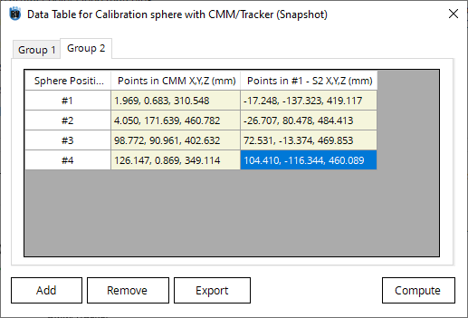
S2-1 (in S2)	1.960, 0.680, 310.540	-17.208, -137.323, 419.117
S2-2 (in S2)	4.050, 171.630, 460.780	-26.707, 80.478, 484.483
S2-3 (in S2)	98.770, 90.960, 402.630	72.531, -13.324, 469.853
S2-4 (in S2)	126.140, 0.860, 349.114	104.410, -116.374, 460.089

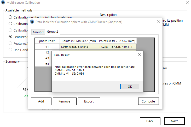
Enter Sensor Type and fill out if there is portable CMM and Hand-Eye calibration result.

Go to Select Method tab, and you can see that two methods are available for the current setup. Select Features/Spheres with CMM/Tracker (Snapshot) and click Next.

Click Add Meas to create a new row. Type in the data collected.

Note

At least 4 positions are required. For better calibration results, users can increase the numbers of spheres or put the spheres as scattered as possible.

Repeat the same procedure for Group 2.

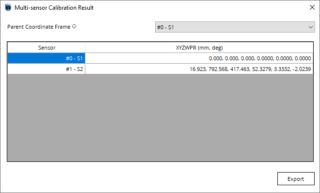
Click Compute. The error and the result is shown.

2.4.7. Intel Realsense sensors with a large box

In this example, two Intel Realsense sensors that have a common FOV are mounted on a rigid fixture. The sensors will be looking at objects that are placed 2 meters away from the sensors, so the regular calibration artifacts are not suitable due to low resolution at far distances.

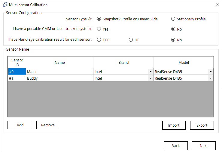
Sensor Name	Model Name
Main	Intel Realsense D435
Buddy	Intel Realsense D435

First, the user needs to prepare a cardboard box that has clearly defined edges and flat surfaces for better results. The user needs to label the box with marks (a circle, a square, and a triangle) as per the image and measure the three dimensions. These marks will later be used to identify the orientation of the box.

Open the toolbox and select Multi-sensor Calibration. Go to Sensor Type and fill out if there is portable CMM and Hand-Eye calibration result.

Go to Select Method tab, select Use a large box for wide FOV snapshot sensors, and click Next.

Put Parent Sensor and Buddy Sensor under Group 1 because they have common FOV and thus they look at the same calibration artifact.

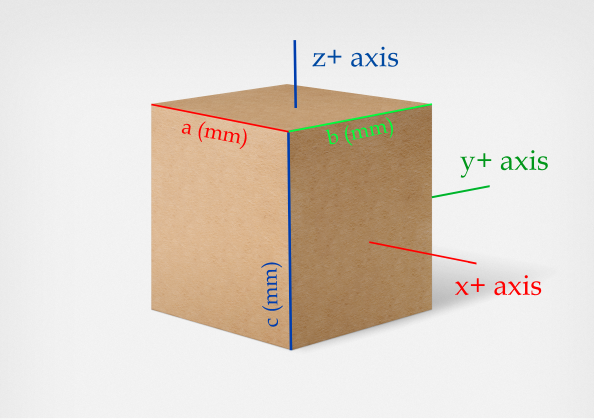
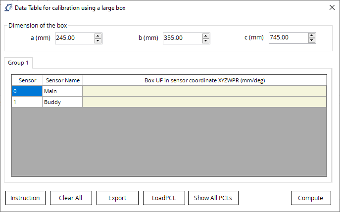
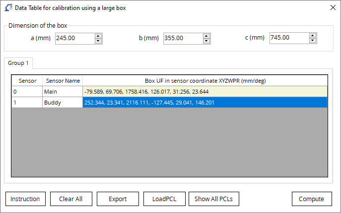
In the data table, the user needs to type in the dimension of the box in mm. Click Instruction button to see the definition of a (mm), b (mm), and c (mm).

For each camera, the user needs to find the UF of the cardboard box in the format of X, Y, Z, W, P, R. The center of the box is defined as the origin and the positice direction of the axes are defined in the schematic diagram.

In our toolbox, we provide a box fitting feature which allows the user to find the UF of the cardboard box with ease. Select a cell and click LoadPCL.

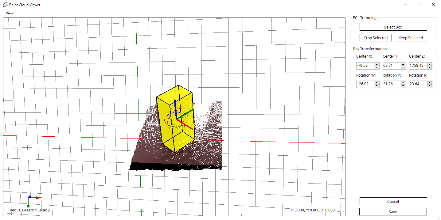
Move and rotate the yellow box to fit the point cloud. The user can either type in the values to the textbox to change the global X, Y, Z, W, P, R, or use the mouse cursor to move the box in its local axis.

Click Save button to transfer the result to the data table. When all cells are filled in properly, the user can click Show ALL PCLs to see if the point clouds are merged properly. If not, the user can go back and redo box fitting. Click Save to see the final result.

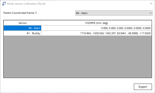
Using the transformation calculated, the point cluods generated by the two sensors can be brought under the same coordinate frame.