6. Linear Slide Calibration Tool

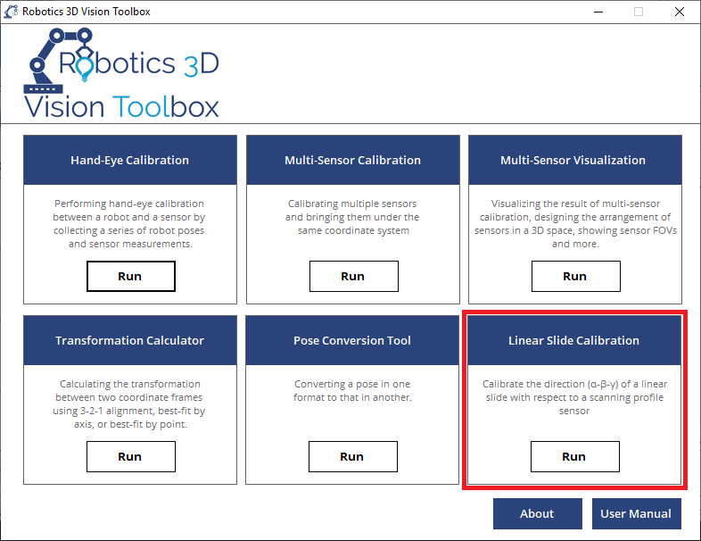
6.1. What is Linear Slide Calibration?

Profile sensors are often mounted on a linear slide to perform inspections. The profiles, either triggered by time or the encoder, are processed to form a 3D point cloud of the objects being scanned.

However, unlike snapshot sensors, profile sensors require extra calibration steps to generate high-accuracy point clouds. For example, we need to know:

• the profile-to-profile distance (encoder calibration).

• the direction of the linear motion with respect to the sensor coordinate (αβγ calibration).

In addition, we need to know how to evaluate the accuracy of the whole system after the calibrations are done. To solve these issues, the Linear Slide Calibration Tool is developed.

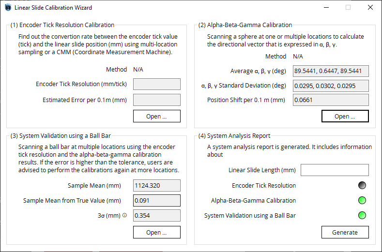
6.2. Linear Slide Calibration Wizard

The Linear Slide Calibration Wizard enables users to perform encoder calibration and αβγ calibration with ease. When these calibrations are done, we can perform a system validation using a ball bar to estimate the error of the whole system. In the end, a report is generated using the system analysis report tool.

6.3. Encoder Calibration

encoder calibration is used when an encoder is used to control the position of the linear slide. In encoder calibration, the parameter being calibrated is the encoder resolution in tick/mm. A well calibrated resoultion can significantly reduce the error and distortion of the generated point cloud from the scanning motion of a laser profile sensor.

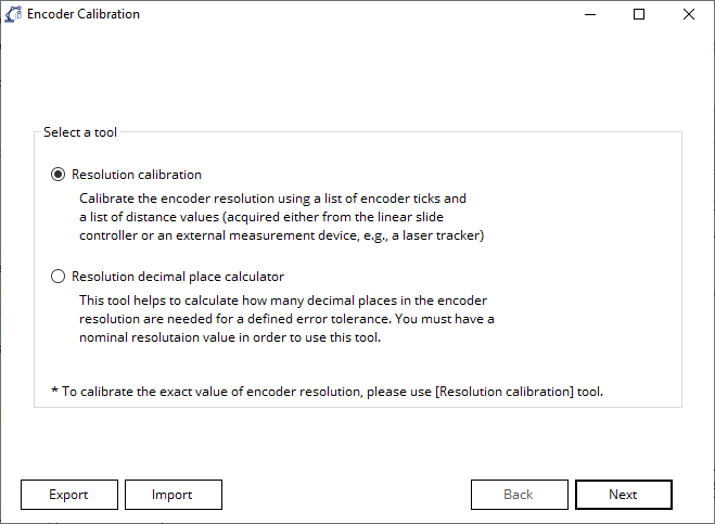
Two calibration modes are supported in encoder calibration: Resolution Calibration and Resolution Decimal place calculator:

• Resolution Calibration: Enter a list of encoder tick values, and the corresponding slide position information (either acquired from the linear slide controller or an external measurement device). The tool will perform a linear regression to calculate the resolution of the encoder resolution.

• Resolution Decimal place calculator: Input the nominal encoder resolution and the required error tolerance. The tool will verify if the resolution is precise enough for the required error tolerance in terms of decimal places.

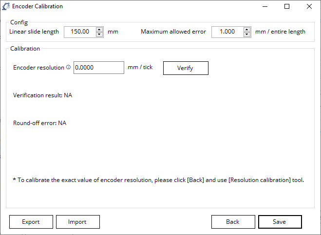
6.3.1. Resolution Decimal place calculator

1. In Config group, enter the Linear Slide Length and Maximum allowed error.

Note

Maximum allowed error is defined as the maximum allowed error in the length of the generated point cloud when scanning over the entire linear slide. E.g., if the linear slide is 1000 mm long and the accuracy requirement is to generate a point cloud of 1000±0.1 mm long when scanning over the entire length, the Maximum allowed error is 0.1 mm.

2. In the Calibration group, enter the nominal Encoder resolution. Make sure all significant figures are entered, so if the resolution is 0.1 mm and accurate up to a hundredth mm, enter 0.10 mm instead of 0.1 mm.

3. Click Verify to verify if the entered resolution is precise enough for the Required error tolerance.

In case the resolution is precise enough, the text below the Verify button will indicate that the resolution is precise enough and show the round-off error (which will be smaller than the Required error tolerance) assuming the entered Encoder resolution is absolutely accurate.

In case the resolution is not precise enough, the text below the Verify button will indicate that the resolution is not precise enough. It will also show the required decimal places to achieve the Required error tolerance and show the round-off error (which will be larger than the Required error tolerance).

4. Click Save to save the calibration result and exit the encoder calibration tool.

6.3.2. Resolution Calibration

1. In Config group, enter the Linear Slide Length and Required error tolerance.

2. In the Calibration group, enter a list of Tick value in the first column, a list of Distance from the linear slide controller. If a more accurate calibrated is to be performed, the user can also deploy an external measurement device, e.g., a laser tracker, the Distance from the measurement device can be input into the third column, but this column is optional.

Note

When filling the table, it is suggested to enter at least ten sample points. The user may evenly select more than ten positions along the length of the linear slide.

3. After filling the table, click Calibrate. A new window will pop-up, showing all data points and the fitted line in one figure. The calibrated resolution and the goodness of fitting will also be shown below the figure. The user may close the window after viewing the fitting result.

4. The calibrated resolution will also be displayed in the textboxes below the table.

5. Click Save to save the calibration result and exit the encoder calibration tool.

6.4. αβγ Calibration

αβγ calibration is used to calculate the direction vector of a linear slide with respect to the profile sensor coordinate frame. This direction vector defines the how these profiles are positioned in the 3D space; the generated point cloud may be distorted if the calibration is not performed properly.

Note

Linear Slide Calibration is required when:

• we use one or multiple stationary profile sensors to scan a part that is transported by a linear slide; or

• we use one or multiple stationary profile sensors that are mounted on a linear slide to scan a stationary part.

The direction vector of the linear slide with respect to a profile sensor is expressed by three angles in degrees. α, β, and γ are the angles between the direction vector of the linear slide and the x, y, and z coordinate of the sensor, respectively.

Warning

The αβγ values are subject to the following restriction to be considered a valid directional vector:

\[cos(α)^2+cos(β)^2+cos(γ)^2=1\]

Here, we will show how αβγ calibration tool can be used for calibrating a profile sensor and a linear slide. Open the αβγ calibration tool from the main wizard window.

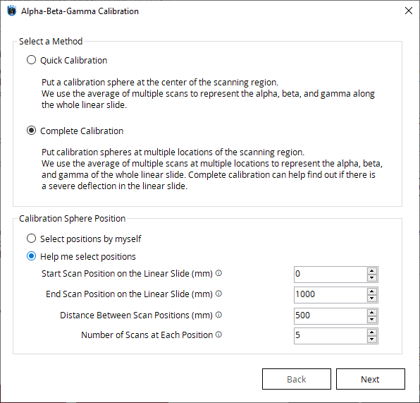
There are 2 ways to perform an αβγ calibration:

• Quick Calibration: Put a sphere artifact at the center of the slide and scan multiple times.

• Complete Calibration: Put a sphere artifact at multiple locations and perform multiple scans at each.

Complete Calibration is recommended if the travelling distance of the linear slide is long (> 1m), or the error of Quick Calibration is large. In this mode, the user can either select locations by themselves, or use the buil-in feature to generate the sphere locations.

Note

Although αβγ calibration is often repeatable, we recommend having 5 scans for each sphere position. Also, if the user wants to perform a copmlete calibration, we recommend having a sphere every 0.5 m.

6.4.1. LMI GoCator 2XXX Series Setting

First, set up the sensor in the LMI web interface. If the user wants to use Encoder Trigger Mode, type in the Resolution (mm/tick). This value can be obtained from the linear slide controlling software, or the Encoder Tick Resolution Calibration in the toolbox (for better accuracy). If the user wants to use Time Trigger Mode, type in the Speed (mm/s).

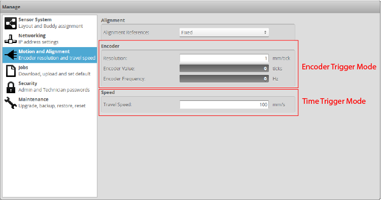
Next, set the Trigger Mode. If the user wants to use Encoder Trigger Mode, type in the spacing (mm). If the user wants to use Time Trigger Mode, type in the Frame Rate (Hz).

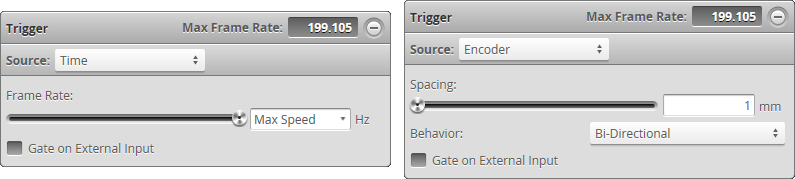
Note

For αβγ calibration we recommend a speed of 50 mm/s for both Encoder Trigger Mode and Time Trigger Mode. Also, if the user is using a BW sphere as the calibration artifcat, we recommend having a profile-to-profile distance of 0.15mm. Therefore, if the user wants to use Encoder Trigger Mode, we recommend setting the spacing (mm) at 0.15 mm. If the user wants to use Time Trigger Mode, we recommend setting the Frame Rate (Hz) to around 300 Hz.

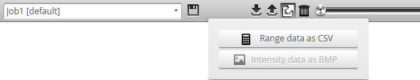
Finally, perform a scan and save the profile to .csv format. Please refer to LMI official manual for instructions.

6.4.2. Quick Calibration

For quick calibration, the user needs to put a sphere in the FOV (Field of View) of the profile sensor. It is better to have the sphere located at the center of the scanning range so that it is a better represenstation of the true value of the αβγ. The image below shows the table for quick calibration.

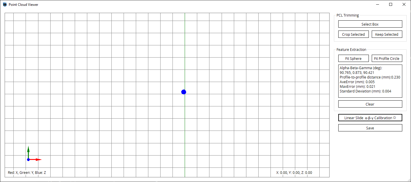
Since the Robotics 3D Vision Toolbox does not communicate with hardware, we need to either rely on the raw data from the profile sensors or 3rd party software to retrieve the point cloud. Here, we show how we can calculate αβγ using a LMI Profile Sensor. Select an empty cell, click Load Pointcloud and slect LMI Profile Sensor (.csv). Select the file generated using the LMI web interface.

In the point cloud viewer, remove irrelevant point clouds and leave the sphere. Select Linear Slide α-β-γ Calibration and check Estimate Profile-to-Profile Spacing.

Note

For best results, it is advised that the sphere is located at the center of the FOV.

The αβγ results are generated in the result text box. Click save and pass the result to the data table.

Warning

In our algorithm, the αβγ result is always close to 90, 0, 90 because we assume the direction is always along the sensor y+. As a result, the user may need to either reverse the encoder polarity or transform the αβγ result to get the correct point cloud.

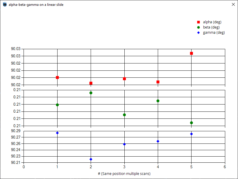
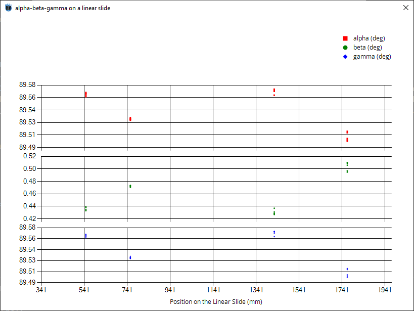
When all data are collected, click Compute to generate the final result and error.

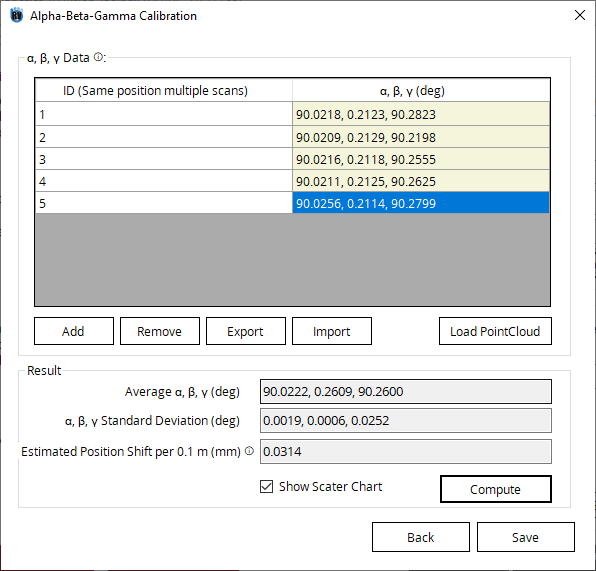
A chart is also generated to view the repeatability of the calibration.

6.4.3. Complete Calibration

Complete Calibration is similar to Quick Calibration except that the user can select the sphere positions by himself. The sphere positions, expressed in mm, are only used when plotting the result in the chart, and it will not affect the accuracy of the calibration. Below is an example of Complete Calibration. To get a reliable result, make sure multiple scan data are collected at the same location.

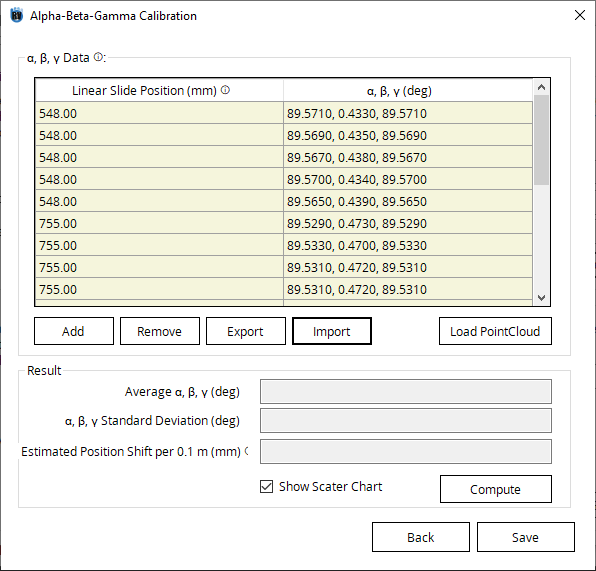
When all data are collected, click Compute to generate the final result and error. A chart is also generated to view the repeatability of the calibration.

Note

Oftentimes, the center of the linear slide has the largest strain and thus the αβγ values might differ from those at other locations.

6.5. System Validation using a Ball Bar

The accuracy of the linear slide system is evaluated using a ball bar. Using the result of encoder calibration and αβγ calibration to scan a ball bar. Type in the true length of the ball bar and the position of each sphere in the table.

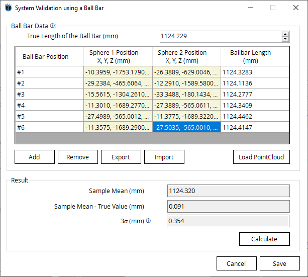
Click Calculate and a plot is generated to show the measurement results.

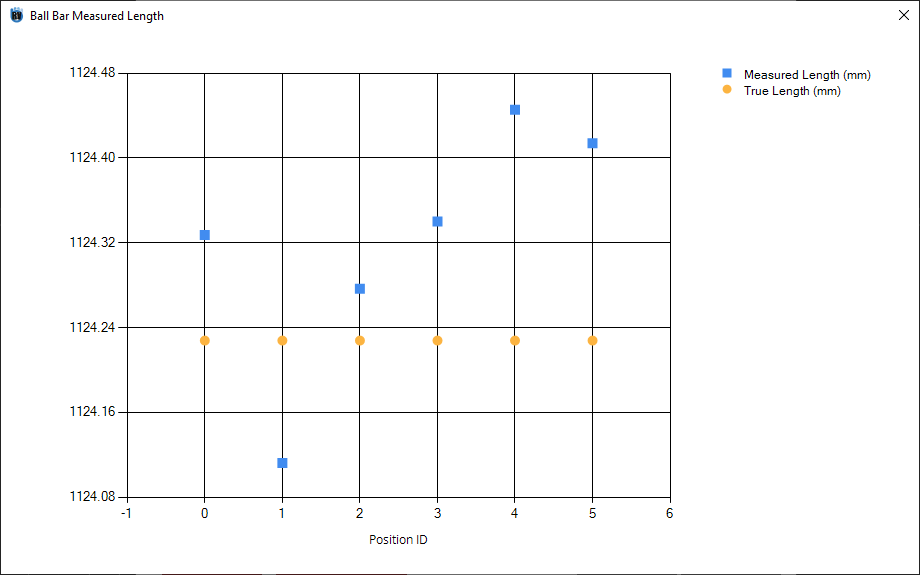
Sample mean (mm), sample mean - true value (mm), 3σ (mm) are provided as metrics for the system accuracy.

6.6. System Analysis Report

After finishing encoder calibration, αβγ calibration, and ball-bar validation, all indication lights in System Analysis Report will turn green, and the user may click generate to generate a complete pdf report of the entire linear slide calibration.

There are 5 chapters in the report.

• Chapter 1 reports all information in encoder calibration.

• Chapter 2 reports all information in αβγ calibration.

• Chapter 3 reports all information in ball-bar validation.

• Chapter 4 provides a thorough error analysis based on the result of encoder calibration, αβγ calibration, and ball-bar validation. Especially, it shows the error contribution of each possible error source in the linear slide system. The user may use these information to identify the source which contributes the most error and thus make changes accordingly. E.g., if encoder resolution round-off contributes most error in terms of percentage, the user may consider redoing the encoder calibration or perferming the calibration with the aid of an external measurement device.

• Chapter 5 is the appendix showing all figures generated during encoder calibration, αβγ calibration, and ball-bar validation.